On March 5, 2010, Mann co-author Bradley filed a plagiarism complaint with George Mason University, alleging that Wegman had copied boilerplate descriptions of proxies from Bradley’s useful but ordinary textbook, which blogger Deep Climate described (incorrectly) as “seminal”. Bradley’s allegations were based on comparisons previously reported by Deep Climate (e.g. link). In a subsequent interview with USA Today, Bradley breathlessly stated:
Clearly, text was just lifted verbatim from my book and placed in the (Wegman) report. Talk about irony. It just seems surreal (that) these authors could criticize my work when they are lifting my words.”
Making Bradley’s allegation even more surreal, it turns out that Bradley’s own description of tree rings as proxies had been copied, including more than a dozen figures and captions almost verbatim, from Harold Fritts’ 1976 textbook, Tree Rings and Climate. Of the first 13 figures in Bradley’s dendro chapter, 12(!) are either copied exactly from Fritts 1976 or, in a few cases, with negligible “paraphrase” (e.g. Bradley Figure 10.10 combines single-columned Fritts Figure 7.10 and 7.11 into a double-columned figure).
In all 12 figures, Bradley copies often lengthy text from Fritts 1976 (in the form of captions). In six of the 12 figures, although the language is taken from Fritts 1976, Bradley cites other provenance for the articles. In each such case, the language in Bradley appears to be a paraphrase of the cited article, while it is, in fact, a copy of the uncited version in Fritts 1976. Since much of Bradley’s dendro chapter is a commentary on the figures from Fritts, Bradley’s text draws heavily on ideas from Fritts 1976, and, in some cases, Bradley’s language tracks Fritts’ rather closely (without specific attribution.) Bradley 1985 included a commendation of Fritts 1976 in its introduction, but this commendation was removed in Bradley 1999.
For the six figures actually referenced to Fritts 1976, the Bradley 1985 captions all conclude with “after Fritts 1976” (“after” is dropped in Bradley 1999). I leave it to readers to comment on whether the term “after” Fritts 1976 fully captures the fact that the figures are in fact identical and the lengthy captions are, in most cases, either verbatim or near verbatim.
In this article, I will compare 12 Bradley 1985 figures and captions to predecessor Fritts figures and captions. In my next article (link), I’ll compare language in the running text. It also turned out that Bradley had an ulterior motive in his plagiarism complaint (see link): Bradley offered to withdraw his plagiarism complaint against Wegman if Wegman withdrew his report from the Congressional record.
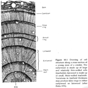
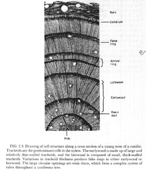
Bradley 1985 Figure 10.1
Bradley 1985 Figure 10.1 is identical to Fritts 1976 Figure 2.3.
Fritts 1976 Figure 2.3: Drawing of cell structure along a cross section of a young stem of a conifer. The earlywood is made up of large and relatively thin-walled cells (tracheids); latewood is made up of small, thick-walled tracheids. Variations in tracheid thickness may produce false rings in either earlywood or latewood.
Bradley 1985 Figure 10.1: Drawing of cell structure along a cross section of a young stem of a conifer. The earlywood is made up of large and relatively thin-walled cells (tracheids); latewood is made up of small, thick-walled tncheids. Variations in tracheid thickness may produce false rings in either earlywood or latewood (after Fritts, 1976).
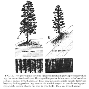
Bradley 1985 Figure 10.2
Bradley 1985 Figure 10.2 is identical to Fritts 1976 Figure 1.5 and Fritts 1971 Figure 3.
The caption to Bradley 1985 Figure 10.2 states:
Trees growing on sites where climate seldom limits growth processes produce rings that are uniformly wide (left). Such rings provide little or no record of variations in climate and are termed complacent. (right): Trees growing on sites where climatic factors are frequently limiting produce rings that vary in width from year to year depending on how severely limiting climate has been to growth. These are termed sensitive (from Fritts, 1971).
The caption to Fritts 1971 Figure 3 is related but not so close:
Trees with ample moisture and favorable temperatures are not limited by climatic factors (left). Their rings are uniformly wide and there is little variation in thickness from one ring to the next. Trees on arid or extremely cold sites may often be limited by climatic factors (right). Their rings are narrow and there may be marked variation in ring thickness corresponding to variations. in climatic factors which have limited growth.
However, the caption to unreferenced Fritts 1976 Figure 1.5 is virtually identical:
Trees growing on sites where climate seldom limits growth processes produce rings that are uniformly wide (A). Such rings provide little or no record of variations in climate and are termed complacent. Trees growing on sites where climatic factors are frequently limiting produce rings that vary in width from year to year depending on how severely limiting climate has been to growth. (B) These are termed sensitive.
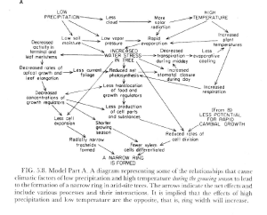
Bradley 1985 Figure 10.3
Bradley 1985 Figure 10.3 is identical to Fritts 1976 Figure 5.8 and Fritts 1971 Figure 5.
The caption to Bradley 1985 Figure 10.3 states:
A schematic diagram showing how low precipitation and high temperature during the growing season may lead to the formation of a narrow tree ring in arid-site trees. Arrows indicate the net effects and include various processes and their interactions. It is implied that the effects of high precipitation and low temperature are the opposite and may lead to an increase in ring widths (from Fritts, 1971).
This is virtually identical to the corresponding caption in Fritts 1976 – Figure 5.8. (Bradley changed “will increase” to “may lead to an increase”.)
Model Part A. A diagram representing some of the relationships that cause climatic factors of low precipitation and high temperatures during the growing season to lead to the formation of a narrow ring in arid-site trees. The arrows indicate the net effects and include various processes and their interactions. It is implied that the effects of high precipitation and low temperature are the opposite, that is, ring width will increase.
The caption to Fritts 1971 Figure 5 is related:
Physiological Model A illustrating how low precipitation and high temperature during the growing season (season of cambial activity) may cause a ring to be narrow for conifers growing on semiarid and warm sites. The climatic conditions affect physiological processes which limit the rate of cell division, the amount of cell expansion or the length of the growing season.
The Bradley language is clearly derived from the language from the unreferenced Fritts 1976.
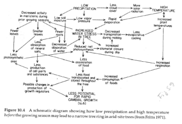
Bradley 1985 Figure 10.4
Bradley 1985 Figure 10.4 is identical to Fritts 1976 Figure 5.9 and Fritts 1971 Figure 6.
The caption to Bradley 1985 Figure 10.4 states:
A schematic diagram showing how low precipitation and high temperature before the growing season may lead to the formation of a narrow tree ring in arid-site trees. (from Fritts, 1971).
The language from the corresponding Figure 5.9 in unreferenced Fritts 1976 is:
Model Part B. A diagram representing some of the relationships that cause climatic factors of low precipitation and high temperatures prior to the growing season to lead to the formation of a narrow ring in arid-site trees. Compare with Fig 5.8.
The language in cited Fritts 1971 Figure 6 is again related but not as close as the unreferenced Fritts 1976:
Physiological Model B illustrating how low precipitation and high temperature prior to the growing season (season of cambial activity) may cause the ring to be narrow for conifers growing on semiarid and warm sites. The climatic conditions may affect physiological processes which precondition the plant, reduce the potential for rapid growth and reduce the rate of cell division (shown in Model A) so that a narrow ring is formed.
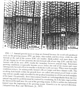
Bradley 1985 Figure 10.5
Bradley 1985 Figure 10.5 is identical to Fritts 1976 Figure 1.5.
The caption to Bradley 1985 Figure 10.5 is copied almost word for word from caption to Fritts 1976 Figure 1.5:
Bradley 1985 Figure 10.5: Annual growth increments or rings are formed because the wood cells produced early in the growing season (earlywood, EW) are large, thin-walled, and less dense, while the cells formed at the end of the season (latewood, LW) are smaller, thick-walled, and more dense. An abrupt change in cell size between the last-formed cells of one ring (LW) and the first-formed cells of the next (EW) marks the boundary between annual rings. Sometimes growing conditions temporarily become severe before the end of the growing season and may lead to the production of thick-walled cells within an annual growth layer (arrows).This may make it difficult to distinguish where the actual growth increment ends, which could lead to errors in dating. Usually these intra-annual bands or false rings can be identified, but where they cannot the problem must be resolved by cross-dating (after Fritts, 1976).
Fritts 1976 Figure 1.5: Annual growth layers or rings are formed because the wood cells produced early in the growing season (EW) are large, thin-walled, and less dense, while the cells formed at the end of the season (LW) are smaller, thick-walled, and more dense. An abrupt change in cell size between the last-formed cells of one ring (LW) and the first-formed cells of the next (EW) marks the boundary between annual rings. Sometimes growing conditions temporarily become severe before the end of the growing season and cause subsequently formed cells to be smaller with thicker walls (arrows). When more favorable conditions return, the subsequently formed cells are larger and have thinner walls. The resulting dark bands within the growth layer are called intra-annual growth bands or false rings and are usually identified by the gradual transition in cell-size on both margins of the band. Occasionally these intra-annual bands are indistinguishable from the true annual ring and the problem must be resolved by crossdating. In A, the false ring is within the latewood formed near the end of the growing season. In B, it is within the earlywood formed near the beginning of the growing season. Growth is in the upward direction. (Adapted from Kuo and McGinnes Jr, 1973).
Bradley 1985 Figure 10.6
Bradley 1985 Figure 10.6 is identical to Fritts 1976 Figure 1.8.
The caption to Bradley 1985 Figure 10.6 is copied almost word for word from caption to Fritts 1976 Figure 1.8:
Bradley 1985 Figure 10.6: Cross dating of tree rings. Comparison of tree-ring widths makes it possible to identify false rings or where rings are locally absent. For example in (A), strict counting shows a clear lack of synchrony in the patterns. In the lower specimen of (a), rings 9 and 16 can be seen as very narrow and they do not appear at all in the upper specimen. Also, rings 21 (lower) and 20 (upper) show intra-annual growth bands. In (b) the positions of inferred absence are designated by dots (upper specimen), the intra-annual band in ring 20 is recognized and the patterns in all ring widths are synchronously matched (after Fritts 1976).
Fritts 1976 Figure 1.8: Cross dating makes it possible to recognize areas where rings are locally absent or where intra-annual growth band appears like a true annual ring. The patterns of wide and narrow rings are compared among specimens. Every fifth ring is numbered in the diagram and in A the patterns of wide and narrow rings match until ring number 9, after which a lack of synchrony in pattern occurs. In the lower specimen of A, rings 9 and 16 can be seen as very narrow and they do not appear at all in the upper specimen; while rings 21 (in the lower) and 20 (in the upper) show intra-annual growth bands. In the upper specimen of B, the positions of inferred absence are designated by two dots, the intra-annual band in ring 20 is recognized and the patterns in all ring widths are synchronously matched (Drawing by M. Huggins).
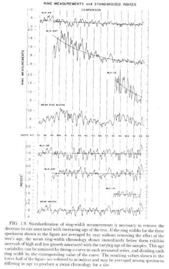
Bradley 1985 Figure 10.7
Bradley 1985 Figure 10.7 is identical to Fritts 1976 Figure 1.9 and Fritts 1971 Figure 2.
The caption to Bradley 1985 Figure 10.7 states:
Standardization of ring-width measurements is necessary to remove the decrease in size associated with increasing age of the tree. If the ring widths for the three specimens shown in the upper figure are simply averaged by year, without removing the effect of the tree’s age, the mean ring-width chronology shown below them exhibits intervals of high and low growth, associated with the varying age of the samples. This age variability is generally removed by fitting a curve to each ring-width series, and dividing each ring width by the corresponding value of the curve. The resulting values, shown in the lower half of the figure, are referred to as indices, and may be averaged among specimens differing in age to produce a mean chronology for a site (lowermost record) ( from Fritts, 1971).
The language from Figure 1.8 in the unreferenced Fritts 1976 version is virtually identical:
Standardization of ring-width measurements is necessary to remove the decrease in size associated with increasing age of the tree. If the ring widths for the three specimens shown in the upper figure are averaged by year, without removing the effect of the tree’s age, the mean ring-width chronology shown immediately below them exhibits intervals of high and low growth associated with the varying age of the samples. This age variability can be removed by fitting a curve to each ring-width series, and dividing each ring width by the corresponding value of the curve. The resulting values shown in the lower half of the figure are referred to as indices and may be averaged among specimens differing in age to produce a mean chronology for a site.
The language in Figure 2 from the citation, Fritts 1971, is again related, but not as close as the unreferenced Fritts 1976:
Standardization is necessary because the first-formed rings are generally wider than those found in the older portions of stems and because some trees grow more rapidly than others. If ring-width measurements, plotted as a function of year of formation (upper plots) are averaged, the mean chronology will show long-term variations arising from differences in ring age and mean growth rate of different sampled specimens (fourth plot). When an exponential curve is fitted as shown in the upper plots and the value of each cure during each year is divided into the ring width for that year, new values are obtained which are referred to as indices (lower plot). These indices do not vary as a function of tree age and mean growth and have an expectation value of 1.0. Such indices may be safely averaged (lowest plot) to obtain a ring-width chronology that is likely to correspond to short-term fluctuations in climate that have limited the growth of the trees.
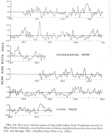
Bradley 1985 Figure 10.9
Bradley 1985 Figure 10.9 is identical to Fritts 1976 Figure 8.8.
The caption to Bradley 1985 Figure 10.9 states:
Five year running means of ring width indices from Pseudotsuga menziesii at Mesa Verde, Colorado, corrected for autocorrelation and plotted on every even year from AD442 through 1962 (after Fritts et al 1965)
The caption to unreferenced Fritts 1976 Figure 6.6 is identical:
Five year running means of ring width indices from Pseudotsuga menziesii at Mesa Verde, Colorado, corrected for autocorrelation and plotted on every even year from AD442 through 1962 (Modified from Fritts et al 1965c)
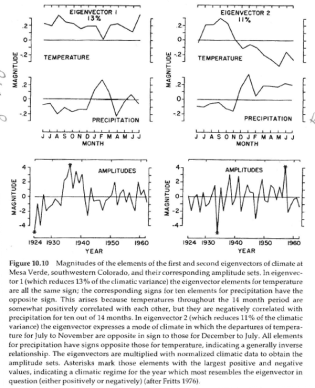
Bradley 1985 Figure 10.10
Bradley 1985 Figure 10.10 is copied from Fritts 1976 Figures 7.10 and 7.11:
The captions are indistinguishable:
Bradley 1985 Figure 10.10: Magnitudes of the elements of the first and second eigenvectors of climate at Mesa Verde, southwestern Colorado, and their corresponding amplitude sets. In eigenvector 1, (which reduces 13% of the climatic variance) the eigenvector elements for temperature are all the same sign; the corresponding signs for ten elements for precipitation have the opposite sign. This arises because temperatures throughout the 14 month period are somewhat positively correlated with each other, but they are negatively correlated with precipitation for ten out of 14 months. In eigenvector 2 which reduces 11% of the climatic variance) the eigenvector expresses a mode of climate in which the departures of temperature for July to November are opposite in sign to those of December to July. All elements for precipitation have signs opposite those of temperature, indicating a generally inverse relationship. The eigenvectors are multiplied with normalized climatic data to obtain the amplitude sets. Asterisks mark those elements with the largest positive and negative values, indicating a climatic regime for the year which most resembles the eigenvector in question (either positively or negatively (after Fritts 1976).
Fritts 1976 Figure 7.10: Plot of the magnitudes of the elements of the first and most important eigenvector of Mesa Verde climate, which reduces 13% of the climatic variance, and the corresponding amplitude set. The eigenvector expresses a mode of climate in which the departures of temperature for July to November are opposite in sign to those of December-July. All elements for precipitation have signs opposite those of temperature, indicating a generally inverse relationship. The eigenvector is multiplied with normalized climatic data to obtain the amplitude set. Asterisks mark those elements with the largest positive and negative values, indicating the most resemblance of the climatic regime for the year to that particular eigenvector. (See Fig 7.9).
Fritts 1976 Figure 7.11: The magnitudes of the elements of the second eigenvector of Mesa Verde climate, which reduces 11% of the climatic variance, and the corresponding amplitude set. The eigenvector elements for temperature are all the same sign; and the corresponding signs for ten elements for precipitation have the opposite sign. This arises because temperatures throughout the 14 month period are somewhat positively correlated with each other, but they are negatively correlated with precipitation for ten out of 14 months. The eigenvector is multiplied with normalized climatic data to obtain the amplitude set. Asterisks mark those elements with the largest positive and negative values, indicating the most resemblance of the climatic regime for the year to that particular eigenvector. (See Fig 7.12).
Bradley Figure 10.11
Bradley 1985 Figure 10.11 copied three of the five panels of Fritts 1976 Figure 7.13.
The captions are indistinguishable:
Bradley Figure 10.11: Response functions obtained from a stepwise regression analysis using amplitudes of eigenvectors to estimate a ring-width chronology representing six Pinus ponderosa sites along the lower slopes of the Rocky Mountains, Colorado. Steps with 1, 3 and 12 predictor variables are shown. Percentage variance reduced can be calculated by multiplying the R2 value by 100. The regression coefficients for amplitudes are converted to response functions though when response functions are complex as in this example, a linear combination of many eigenvectors is needed to obtain the best fitting relationship (after Fritts 1976).
Fritts 1976 Figure 10.11: Response functions obtained from a stepwise regression analysis using amplitudes of eigenvectors and prior growth to estimate a ring-width chronology representing six Pinus ponderosa sites along the lower slopes of the Rocky Mountains, Colorado. Steps with 1, 3, 7, 12 and 20 predictor variables are shown. The regression coefficients for amplitudes are converted to response functions (Equation 7.22) . When response functions are complex as in this example, a linear combination of many eigenvectors is needed to obtain the best fitting relationship. Prior growth was entered into regression after the step with 12 variables. The percent variance can be calculated by multiplying the R2 by 100.
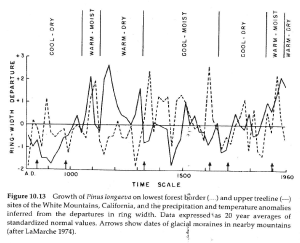
Bradley Figure 10.13
Bradley 1985 Figure 10.13 is identical to Fritts 1976 Figure 8.9 and Lamarche 1974 Figure 6.
The caption to Bradley 1985 Figure 10.13 states:
Growth of pinus longaeva on lower forest border (…) and upper treeline (—) sites of the White Mountains, California, and the precipitation and temperature anomalies inferred from the departures in ring width. Data expressed as 20 year averages of standardized normal values. Arrows show dates of glacial moraines in nearby mountains (after Lamarche 1974)
The caption to Fritts 1976 Figure 8.9 is virtually identical:
The 20-year average growth , expressed in standardized normal values, in Pinus longaeva on lower forest border (…) and upper treeline (—) sites of the White Mountains, California, and the precipitation and temperature anomalies inferred from the departures in ring width. Arrows show dates of glacial moraines in nearby mountains (From Lamarche, V.C. 1974 Science 183 (4129) 1043-1048, copyright 1974 by the American Association for the Advancement of Science.)
The caption to Lamarche 1974 Fig 6 is related, but not nearly as close as the unreferenced Fritts 1976:
Departures from mean growth(normalized 20-year means) trees on ecologically contrasting sites in the White Mountains and inferred climatic anomalies. Arrows show dates of glacial moraines in the nearby Sierra Nevada (19); all except the youngest were formed during periods judged to be relatively cool from the tree-ring evidence. Glacial advances of the early 1300s and early 1600s also coincide with unusually wet periods.
analogous to the stepwise regression coefficients described in the previous section…
Needless to say, there are many other examples.
Note: Edited on December 12, 2023 to streamline presentation.
