Lehman Bros. and Consensus

My interest in climate change derived in part from experience in the stock market where “consensus” is not infrequently established in favor of opinions that are completely incorrect. And, in many cases, the people promoting the views are competent and serious people. How are such things possible? I read about the Bre-X and Enron failures, trying to distinguish between the “shame on you” and the “shame on me” components – i.e. yes, the original misconduct and deceit was deplorable; but at what point should proper independent due diligence have been able to detect misconduct? At what point were regulatory agencies negligent? Obviously we’re going to see a new spate of such inquiries in the wake of the recent collapses.

I was particularly intrigued in the cases of Bre-X and Enron failures by the tremendous acolades meted out to the promoters right up to the eve of their collapses.

As evidence of this ongoing interest, a reflection on Bre-X was one of the very first Climate Audit posts (Feb 6, 2005). I observed that Felderhof and de Guzman were lionized at the 1997 PDA convention (March 10-16, 1997) and walked around like royalty only a few days before the fraud was revealed. de Guzman literally disappeared a few days later, supposedly either jumping or being pushed from a plane over the Indonesian jungle. Others speculate that he may have assumed a new identity in a Third World barrio somewhere. The “consensus” disappeared quickly. Take a look at the post.

In another early post, I observed the “consensus” that Enron was not only a well-managed company, but the most outstandingly managed company in the U.S., citing a couple of quotes from Kurt Eichenwald’s Conspiracy of Fools:

The next morning just after ten, Skilling stood beside Lay as a photographer snapped their pictures for an article in Fortune. They were more than happy to participate; already that year, in its annual rankings, Fortune had hailed Enron as America’s best-managed company, knocking General Electric from the number-one perch. (p.227)

After months of effort, Karen Denne from Enron’s public relations office landed the big fish: CFO magazine had selected Fastow as one of the year’s best chief financial officers. (p. 260)”

Lay opened his briefcase and pulled out the latest issue of CFO magazine, glacing at the cover. The Finest in Finance. Lay smiled to himself. He found the table of contents, looking for Fastow’s name. Beneath it were the words: How Enron financed its amazing transformation from pipelines to piping hot. Lay turned to the article, “When Andrew S Fastow, the 37-year old CFO of Enron Corp. boasts that “our story is one of a kind’ he’s not kidding" it began”. Fastow was obviously as creative and sharp as Lay and Enron’s board of directors had come to believe” (p. 267)

Turning now to Lehman Bros. I looked quickly at their website this morning, which reports that in the last two years, Lehman Bros has been ranked #1 by both Barron’s and Fortune:

2006 – Ranks #1 in the Barron’s 500 annual survey of corporate performance for the largest companies in the U.S. and Canada.

2007 – Lehman Brothers ranks #1 “Most Admired Securities Firm” by Fortune.

One more example of “consensus”.

I don’t want readers to start piling on with accusations or making uninformed comparisons of climate change to these corporate failures. For once, I want to be able to be nuanced statements without provoking a lot of piling on. I personally am unimpressed by “consensus”, especially when there is no independent due diligence. That doesn’t mean that I’m impressed by “skeptic” proposals either (BTW).

One of the curious aspects to Enron’s rise to prominence is that nobody understood how they actually made money. That’s one of the reasons why I’m so adamant about wanting clear A-to-B explanations of how doubled CO2 leads to 3 or more deg C and why excuses for not providing such explanations are so disappointing. I believe that forcing oneself to provide such an explanation would be very healthy for the AGW community.

In passing, recall that Enron had an early interest in climate change policy. I was prudent enough to save a pdf of their policy position, which I reported on a couple of years ago.

Lehman Bros also seem to have been actively interested in climate change, producing a couple of reports, most recently here dated Sept 2007. In their acknowledgements, they thank James Hansen for clearing up some “questions that had been niggling us”:

On the scientific side, we are grateful to Dr. James Hansen, Director of the NASA Goddard Institute for Space Studies, who, at the end of a particularly informative dinner hosted by Ben Cotton of the Man Group, gave generously of his time to clear up a number of scientific questions that had been niggling us. Dr. Peter Collins and Richard Heap of the Royal Society provided valuable input and brought us up to date on the more controversial areas of scientific developments in the domain of global climate change.

In the summer and September of 2007, we also spent a lot of time trying to understand “questions that had been niggling us” – like what data set was used in GISTEMP, why Hansen changed the provenance of GISTEMP data sets, how GISTEMP adjustments were done and why. Hansen was notably uncooperative, even saying that he refused to “joust with jesters”. Maybe we went about it the wrong way. Maybe we should have asked Lehman Bros to find out for us.
Hansen's Kingsnorth Testimony

A reader writes in about Hansen’s submission at the Kingsnorth trial. I’m posting up a thread under a couple of conditions. Hansen’s take on scientific matters is influential and important and discussion of scientific topics will be permitted. Please do not post on anything that remotely touches on policy. Please do not make posts complaining or whining about Hansen or AGW or alarmism or anything like that. I’m not going to bother snipping, I’m just going to delete posts that don’t comply. Using words like Cenozoic in the post is encouraged.

Is Steve or anyone interested in taking a look at Hansen’s written submission in the Kingsnorth trial?

It’s online here:

Click to access hansen.pdf

Excerpts from his Q & A are here:

http://www.greenpeace.org.uk/blog/climate/kingsnorth-day-three-trial-jim-hansen-20080903

Written statements from the other defence witnesses are here:

http://www.greenpeace.org.uk/blog/climate/kingsnorth-trial-witness-statements-full-20080912

My Erice Presentation

On Sep 2, I was getting ready to report on my trip to Italy and my presentation to the World Federation of Scientists seminar in Erice, Sicily, when I was rudely interrupted by the publication of Mann et al 2008. It will take time to fully parse the situation, but the main framework is pretty clear. The addiction of Mann and the paleoclimate community to problematic Graybill bristlecone chronologies has not been cured. Indeed, Mann et al 2008 has made things worse, using even more fanciful data sets, such as serial (4 time) use of disturbed Kortajarrvi lake sediments.

I found the Erice conference very interesting. The topics were much more policy-oriented than I try to cover at the blog (climate was only one of many topics, others included energy supply, nuclear security, computer security). Over the next few months, I’ll relax these policies for some individual threads and pick up some of the themes at the conference, as these will undoubtedly be of interest to many readers – indeed, most of the themes will be of more interest to readers than the technical issues that I like to discuss.

But for today, you’ll have to content yourselves with my presentation. I had to submit a written paper and had a 20-minute talk. The presentation immediately prior to mine had used the HS (the IPCC 2001 version) as an unannotated “fact”, which was a good set-up for my presentation. The Erice conferences have a distinguished history of promoting openness in science even (and perhaps especially) in nuclear topics and I think that it was disappointing to many of them that climate scientists, of all people, should be anything less than 100% forthcoming with the provision of data and methods, and the idea of a climate scientist using personal Intellectual Property Rights as a pretext for refusing data and methods definitely did not sit well with scientists from other disciplines who are concerned, as citizens, about quantifying climate change.

Here is the written submission. Most readers here are familiar with the history of the dispute, but third parties aren’t and, points of detail such as different versions of Tornetrask, Polar Urals and Sheep Mountain obviously make no sense except in the context of an ongoing dialogue.

I then proceeded to discuss two problems which between the two of them, pretty much eviscerate all the IPCC AR4 reconstructions: (1) the divergence problem; and (2) differences between updated and IPCC versions of key sites (Tornetrask, Polar Urals and bristlecones). CA readers are familiar with these points, but I made new graphics in a consistent format illustrating the argument, which is pretty simple.

New versions of three important sites (Grudd’s Tornetrask, the unpublished Polar Urals update and Ababneh’s Sheep Mountain) have materially different MWP-modern differentials than the older versions used in the IPCC spaghetti graph (Briffa’s Tornetrask and Yamal; Graybill’s Sheep Mt/Mann’s PC1). Because so many purportedly “independent” studies are not actually “independent”, changes at only three sites cause a reversal of the MWP-modern relationship in 9 of 10 studies in the IPCC spaghetti graph and make the specific IPCC claim of AR4 unsupportable within their likelihood definitions. Here is the conclusion of my paper:

Although the statistical problems of the Mann et al (1998, 1999) reconstruction are by no means conceded within the reconstruction community, they have nonetheless been
identified for some time. Two blue ribbon U.S. panels have acknowledged these
criticisms, but IPCC 2007 did not.

Updated versions of Tornetrask, Urals and Sheep Mountain have opposite medievalmodern
differentials to the IPCC versions. Because virtually all of the IPCC reconstructions rely on these three sites and because the framework of MWP proxies in IPCC reconstructions is so limited, changes in only 3 site versions turn out to have a knock-on impact on 9 of 10 reconstructions, an issue which also affects the Mann et al 1999 reconstruction additional to all the other problems. IPCC failed to provide any accounting or reconciliation of the discrepant versions.

Adding to the problems of the IPCC 2007 reconstructions is the “Divergence Problem” – ring widths going down in the last half of the 20th century, while temperatures go up. In the absence of any such explanation and reconciliation, IPCC could not state within its probability definitions that: “[It is] likely that this 50-year period was the warmest Northern Hemisphere
period in the last 1.3 kyr.”

Verification of paleoclimate studies has been made far more onerous than necessary, by
the failure of authors to archive data and to properly document methodological procedures. Econometrics journals have dealt with similar problems by requiring authors to archive data (as used with accurate data citations to the precise version) and source code as a condition of reviewing. This procedure is recommended for paleoclimate journals as well. In addition, the U.S. National Science Foundation (NSF) has essentially abandoned its duties to ensure that paleoclimate authors comply with existing U.S. data archiving policies and many problems could be averted merely by NSF carrying out its duties.

BBC "Climate Wars"

A placeholder thread.

Mann 2008: the Bristlecone Addiction

I see that the BBC is taking the position that the “evidence” of an MWP-modern differential now is confirmed in so many “independent” studies that the matter is now “incontrovertible”. However these studies are not “independent”; the vast majority of the “independent” studies use the same stale proxy data. In my Erice presentation (which I’ll post up in a day or two), I showed the difference between updated versions of the Tornetrask, Polar Urals and Sheep Mountain data and the older versions used in Team studies, observing that use of the updated versions altered the medieval-modern differential in 9 of 10 canonical studies (the issues in Moberg involve a couple of different proxies, but are similar.)

In regards to the MWP-modern differential, Mann et al 2008 is once again not “independent” of the other studies – the entire suite of Graybill strip bark bristlecones rear up once again. Very few of the “new” proxies covering the MWP contain a relevant HS shape and there are fatal problems with the ones that do (e.g. the Korttajarvi sediments) making one question why these sediments are used in a supposedly serious study.

In a previous post, I made a flash summary of the non-dendro proxies in Mann et al 2008 and I urge interested readers to review that post.

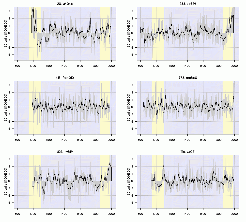
Today I’m providing a flash summary of all the dendro series with SI start dates prior to 1010. While there has been considerable discussion of the use of “tree ring” series in Mann et al 2008, the real issue is the use of Graybill strip bark chronologies, which continue to be used without apology or discussion as to their validity. In the flash image, the HS shaped series labeled as ca534, nv…, co524 etc are invariably Graybill bristlecone strip bark chronologies. The version showed below are non-infilled in the latter portion. Other non-“independent” proxies used over and over are Briffa’s Tornetrask, the Jacoby-d’Arrigo Mongolia series. There is remarkably little that is both new and relevant to a modern-medieval differential, despite the puff.

The continued use of the questionable Graybill strip bark chronologies is highly objectionable, especially in view of Abaneh’s inability to replicate the most important Graybill chronology (ca 534.) It is also objectionable in view of the following puff by Mann et al:

We were guided in this work by the suggestions of a recent National Research Council report (35) concerning an expanded dataset, updated data, complementary strategies for analysis, and the use of thoroughly tested statistical methods.

As has been widely observed, the NRC panel recommended that “strip bark” chronologies be “avoided” in temperature reconstructions – a suggestion obviously not adhered to by the Mann group. This is doubly disappointing as the chairman of the NAS panel, Gerry North, is said to have been a reviewer of the Mann et al 2008 paper, but he seems to have taken no steps whatever to ensure that strip bark chronologies were avoided, though this issue should have been on his mind.


Figure 1. Mann 2008 Dendro proxies standardized to 1400-1980 with 21 year smooth illustrated. Non-infilled. There is one series in the list that doesn’t go back to 1010, but this appears to be an error in the underlying SI and has been left in.

The Pea under the Thimble
The Mann study claims that they can “get” a HS shape without dendro (i.e. without Graybilll bristlecones):

When tree-ring data are eliminated from the proxy data network, a skillful reconstruction is possible only back to A.D. 1500 by using the CPS approach but is possible considerably further back, to A.D. 1000, by using the EIV approach. We interpret this result as a limitation of the CPS method in requiring local proxy temperature information, which becomes quite sparse in earlier centuries. This situation poses less of a challenge to the EIV approach, which makes use of nonlocal statistical relationships, allowing temperature changes over distant regions to be effectively represented through their covariance with climatic changes recorded by the network.

A skillful EIV reconstruction without tree-ring data is possible even further back, over at least the past 1,300 years, for NH combined land plus ocean temperature (see SI Text). This achievement represents a significant development relative to earlier studies with sparser proxy networks (4) where it was not possible to obtain skillful long-term reconstructions without tree-ring data.

But watch the pea under the thimble: the completely defective Korttajarvi sediment chronologies are used in the comparandum series. Yes, the anthropogenically disturbed sediments have a HS pattern, but so what? Surely no one can seriously argue that this presents valid evidence on the modern-medieval differential (whichever way it goes.)

As noted before, in the SI to Mann et al 2008, they purported to account for the defective Korttajarvi sediments by doing a sensitivity analysis without them. But once again, watch the pea under the thimble: the Graybill strip bark chronologies are used in this comparison. Mann et al:

We therefore performed additional analyses as in Fig. S7, but instead compaired the reconstructions both with and without the above seven potentially problematic series [including the four Korttajarvi series], as shown in Fig. S8.

As far as I can tell, this is not a comparison of non-dendro proxies with and without the defective Kortaajarvi series, but before and after of a network which has multiple Graybill bristlecones in the network.

This is what passes as “incontrovertible” evidence in climate science.

Mann 2008: Impact of the Missing Data

Jeff Id has an interesting post in which he examines the 148 “missing” series. Check it out. I haven’t verified the calculation, but will do so. I submitted a comment at his blog observing that the two “Fisher” series are actually Dahl-Jensen borehole reconstructions from Greenland. These two series were said to have been used in Mann and Jones 2003, but the construction of the Mann and Jones 2003 composite is, at present, remains considerably more mysterious than MBH.

Will the Real Slim Shady Please Stand Up? Re-Mix.

There’s an amusing little incident with the deleted “original” data set that was posted up for a few minutes at Mann’s website – you know, the data set that was first demonstrably referenced by a CA reader in the early morning of Sep 5. (I’ll reserve comment for now on issues relating to the timestamp of this data set and the Gavin Schmidt hyperlink to it, presently pointing to a data version that did not exist at the time that the hyperlink was supposedly created.)

Within a day, on the afternoon of Sep 5, the data set was deleted and replaced with another data set, again without notice, in a bewildering concatenation of replacements that is reminiscent of our experience with the Hansen’s GISS data almost a year to the day ago. However, both myself and others took the precaution of downloading the Sep 4 version as soon as we saw it – just in case it disappeared. Not an imprudent precaution, given its almost immediate deletion.

I’ve now had an opportunity to forage through the deleted version. The deleted data had 1357 series, from which 148 series were deleted to yield the 1209 series that now appear in the “original” data. But surely the 1357 series is “more” original than the 1209 series? What criteria were used to winnow out the 148 removed series? Inquiring minds want to know. There’s not a whisper on this topic in the paper or in the SI and, of course, all traces of the 148 series were ruthlessly scrubbed from Mann’s website.

Surprisingly, on the list of deleted series was a series entitled “Yamal 2002”. Now Yamal is very familiar to CA readers, as Briffa replaced the Polar Urals update (with a high MWP) with his Yamal version (with a HS) and this one substitution affects a number of reconstructions (discussed on many occasions:

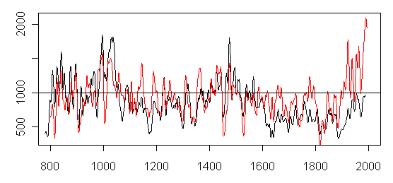
The graphic below illustrates the difference between the Polar Urals update (black) and Yamal (red) (See above links for the impact of the Yamal substitution on the Briffa 2000 reconstruction, a spaghetti graph)


Figure 1. Comparison of Polar Urals update to the Briffa Yamal version.

So why was this series excluded from Mann et al 2008? And if it was no good for Mann et al 2008, why is it any good in the “other” studies?

Just for fun, I plotted up the Mann 2008 version of Yamal (shown in the graphic below):


Figure 2. Plot of “Yamal 2002” in deleted Mann et al 2008

Quite obviously this data set doesn’t have a HS and doesn’t look anything like the Briffa version of Yamal. Where did it come from? This data version is the Yamal version from the original authors (available at WDCP here ). This version matches the graphic in Hantemirov 2002. (In passing, I’ve observed previously that Juckes et al and other Team articles have cited Hantemirov, when they actually used a Briffa version that is not located at WDCP.)

Where did the Briffa Yamal version come from and why is it different than Hantemirov’s? Presumably they use different standardization methods, but then one would have to see the measurement data, which Briffa thus far has steadfastly refused to disclose (for 8 years and multiple articles.)

I still don’t know why the Hantemirov version wasn’t used in Mann et al 2008. Would it “matter”? Yes and no. As a single series, it wouldn’t necessarily “matter”, but it would be nice to know why these series were excluded. Curiously, Mann used Briffa’s Tornetrask version (not Grudd’s), so it’s not like he refused to use grey Briffa versions. It’s odd that the Hantemirov version got into the mix in the first place.

Now there’s a nice little ending to this story. The “wrong” data set – the one deleted from Mann’s website – is the one that Mann sent to WDCP, an archive of record, where Mann can’t change “inconvenient” data sets without leaving a trace. So WDCP has one “original” data set and Mann’s website has another.

Will the real Slim Shady please stand up? (Re-Mix).

Ian Jolliffe Comments at Tamino

Ian Jolliffe, a noted principal components authority, has posted a comment at Tamino’s, which repudiates Tamino’s (and Mann’s) citation of Jolliffe as a supposed authority for Mannian PCA. He wrote to me separately, notifying me of the posting and authorizing me to cross-post his comment and stating that we had correctly understood and described his comments in our response here: :

I looked at the reference you made to my presentation at http://www.uoguelph.ca/~rmckitri/research/MM-W05-background.pdf *after* I drafted my contribution and I can see that you actually read the presentation. You have accurately reflected my views there, but I
guess it’s better to have it ‘from the horse’s mouth’.

Here is Jolliffe’s comment in full:

Apologies if this is not the correct place to make these comments. I am a complete newcomer to this largely anonymous mode of communication. I’d be grateful if my comments could be displayed wherever it is appropriate for them to appear.

It has recently come to my notice that on the following website, http://tamino.wordpress.com/2008/03/06/pca-part-4-non-centered-hockey-sticks/ .. , my views have been misrepresented, and I would therefore like to correct any wrong impression that has been given.

An apology from the person who wrote the page would be nice.

In reacting to Wegman’s criticism of ‘decentred’ PCA, the author says that Wegman is ‘just plain wrong’ and goes on to say ‘You shouldn’t just take my word for it, but you *should* take the word of Ian Jolliffe, one of the world’s foremost experts on PCA, author of a seminal book on the subject. He takes an interesting look at the centering issue in this presentation.’ It is flattering to be recognised as a world expert, and I’d like to think that the final sentence is true, though only ‘toy’ examples were given. However there is a strong implication that I have endorsed ‘decentred PCA’. This is ‘just plain wrong’.

The link to the presentation fails, as I changed my affiliation 18 months ago, and the website where the talk lived was closed down. The talk, although no longer very recent – it was given at 9IMSC in 2004 – is still accessible as talk 6 at http://www.secamlocal.ex.ac.uk/people/staff/itj201/RecentTalks.html
It certainly does not endorse decentred PCA. Indeed I had not understood what MBH had done until a few months ago. Furthermore, the talk is distinctly cool about anything other than the usual column-centred version of PCA. It gives situations where uncentred or doubly-centred versions might conceivably be of use, but especially for uncentred analyses, these are fairly restricted special cases. It is said that for all these different centrings ‘it’s less clear what we are optimising and how to interpret the results’.

I can’t claim to have read more than a tiny fraction of the vast amount written on the controversy surrounding decentred PCA (life is too short), but from what I’ve seen, this quote is entirely appropriate for that technique. There are an awful lot of red herrings, and a fair amount of bluster, out there in the discussion I’ve seen, but my main concern is that I don’t know how to interpret the results when such a strange centring is used? Does anyone? What are you optimising? A peculiar mixture of means and variances? An argument I’ve seen is that the standard PCA and decentred PCA are simply different ways of describing/decomposing the data, so decentring is OK. But equally, if both are OK, why be perverse and choose the technique whose results are hard to interpret? Of course, given that the data appear to be non-stationary, it’s arguable whether you should be using any type of PCA.

I am by no means a climate change denier. My strong impressive is that the evidence rests on much much more than the hockey stick. It therefore seems crazy that the MBH hockey stick has been given such prominence and that a group of influential climate scientists have doggedly defended a piece of dubious statistics. Misrepresenting the views of an independent scientist does little for their case either. It gives ammunition to those who wish to discredit climate change research more generally. It is possible that there are good reasons for decentred PCA to be the technique of choice for some types of analyses and that it has some virtues that I have so far failed to grasp, but I remain sceptical.

Ian Jolliffe

As an editorial comment, the validity of Mannian PCA is only one layer of the various issues.

For example, Wahl and Ammann approach the salvaging of Mann overboard from a slightly different perspective than Tamino. Their approach was to argue that Mannian PCA was vindicated by the fact that it yielded a high RE statistic and thus, regardless of how the reconstruction was obtained, it was therefore “validated”. I don’t see how this particular approach circumvents Wegman’s: “Method Wrong + Answer ‘Right’ = Incorrect Science”, but that’s a different argument and issue. Also if you read the fine print of Wahl and Ammann, the RE of reconstructions with centered PCA are much lower than the RE using incorrect Mannian PCA, but, again, that is an issue for another day.

It would be nice if Jolliffe’s intervention were sufficient to end the conceit that Mann used an “alternate” centering convention and to finally take this issue off the table.

Proxy Screening by Correlation

I’ve made histograms of reported proxy correlations for 1850-1995, as reported in r1209.xls (which contains results for all proxies, unlike SI SD1.xls which withholds results below a benchmark.) The breaks are in 0.1 intervals. On the left is the histogram before screening; on the right, a histogram of the 484 proxies after screening.


Clearly a great deal of analysis could be done on this topic. I’ll just scratch the surface on this, as I’m going to be away for a couple of days, but felt that the issue warranted being on the table right away.

The first couple of things that struck me about the pre-screening distribution were –
1. there was odd tri-modality to the distribution, with a bulge off to the right with very high correlations;
2. the distribution was surprisingly symmetric other than the right-hand bulge, but was “spread” out more than i.i.d. normal distributions;
3. Mannian screening was, for the most part, one-sided, although high negative values were retained.

A little inspection showed that the right-hand bulge of very high correlations arose entirely from the Luterbacher gridded series, which, as I understand it (and I haven’t reviewed the Luterbacher data), contains instrumental information in the calibration period and is not a “proxy” in the sense of tree rings or ice cores. So when Mann says that 484 series passing a benchmark is evidence of “significance”, this inflates the perceived merit of tree ring and ice core data since the 71 Luterbacher series make a non-negligible contribution. Removing the Luterbacher series, one gets the more symmetric distribution shown below:

Next, the bimodality of this distribution calls for a little explanation. The vast majority of the proxies in this figure are tree rings, so we’re back to tree rings. It’s possible that this bimodality is a real effect, i.e. that some chronologies respond negatively to temperature and others positively. But it’s equally possible that a form of pre-screening has already taken place in collating the network with very “noisy” chronologies being excluded from even the pre-screened network. It would take some careful analysis of the tree ring networks to pin this down, but selection bias seems more likely to me than actual bimodality, but that’s just a guess right now.

Next, the correlations are more spread out than one would expect from i.i.d normal distributions, where Mann’s SI states that 90% of the proxies would be within -0.1 to 0.1 correlations. Given the fact that there are almost as many negative as positive correlations, this suggests to me that the effect of autocorrelation is substantially under-estimated in choosing 0.1 as a 90% standard. Given the relatively symmetric distribution, it looks far more likely to me that autocorrelation effects are wildly under-estimated in his benchmark and that the 90% benchmark is much higher. It’s not nearly as clear as Mann makes out that the yield of 484 proxies (less 71 Luterbacher) is as significant as all that.

This particular operation looks more and more like ex-post cherry picking from red noise (along the lines of discussions long ago by both David Stockwell and myself.) This is a low-tech way of generating hockey sticks, not quite as glamorous as Mannian principal components, but it “works” almost as well.

It’s pretty discouraging that Gerry North and Gaby Hegerl were unequal to the very slight challenge of identifying this problem in review.

Borehole Inversion Calculations

Phil B writes:

My day job does include parameter and state estimation using Least Squares and Kalman filtering.

I have replicated several of the non-ice borehole temperature reconstructions and I’ll “share” my observations. The inversion problem boils down to finding the solution to the inconsistent set of linear equations Ax~b, where A is a skinny matrix (mxn) whose columns are generated from the solution of the heat conduction equation. x is a nx1 solution vector where the first two elements are a slope and intercept and the remaining elements are the temperature reconstruction. The b mx1 vector is the borehole temperature profile. The solution is calculated using the pseudo inverse based on the singular value decomposition (svd) where A = U*S*V’ and where U (mxm) and V (nxn) are complete orthonormal basis sets. The A matrix is ill-conditioned with ratio of max to min singular value on the order of 1e6 to 1e7 on the boreholes I replicated. In the older literature only singular values of greater than 0.3 are used in the pseudo inverse, with recent literature using a ridge regression that optimizes the norm of the residual versus the norm of the solution. If you keep singular values that are less than 0.3, the reconstruction is physical unreasonable, i.e. pulses on the order of 20-40 deg K. For 500 year reconstruction and 100 year steps, the 3 smallest singular values out of the seven total aren’t used in the psuedoinverse.

So what is the problem??? The ill-conditioning of A!! For instance if A is rank deficient i.e. rank = n-1, then one has a single null vector z such that A*z = 0_mx1 and an infinite number of solutions for x. For our A, there are 3 “almost” null vectors which are the last three columns of V. So A*v(5), A*v(6), A*v(7)~0_mx1. Let x_est be the pseudo inverse solution using only singular values greater than 0.3. Let’s create a new solution x_new = x_est + 2*v(7). The individual residual changes are on the order of millikelvins. x_new “looks” substantial different then x_est but the values are reasonable. The point is that there are many x_estimates and many reasonable temperature reconstructions that have residuals that are almost identical, with differences that are less then the temperature sensor noise level.

Summarizing, the columns of the ill-conditioned A matrix are created using solutions to the heat conducting equation. x_est is one of many possible temperature histories.