UC inquired about the variance adjustment in Osborn et al (Dendrochronologia 1998), which is used in many Team publications. The number of series in many reconstructions declines as you go back in time. If you take an average of standardized series (the CVM method), the variance over an early time interval will be larger than the variance in a later time period.) The BO variance adjustment was used originally in proxy reconstructions but this procedure or a variant seems to have been introduced into some of the CRU temperature gridcell series as well. The adjustment is described as follows:
Each regional mean thus obtained tended to have greater variance during years when few chronologies were available to contribute to the average; this effect was corrected for by scaling by the square root of the effective number of independent samples available in each year.
First they state
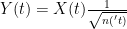
Let’s assume that one starts with a set of series all standardized to 0 mean and sd -1. Then if  is the average of n series with a mean correlation
  ,
,
(1) 
If the series are uncorrelated ( , the variance goes down to 1/n;
(2) 
whereas if the series are perfectly correlated (  ), the variance stays at 1. They assert:
“an artificial signal will be introduced into the variance of Xbar if the sample size varies through time.”
Comparing (1) and (2), they define the “effective independent sample size” as follows:
(4)  ;
;
They express (1) as follows
(5) 
When one thinks about this, this is a very odd terminology. This is measuring not so much the “independent sample size” as the relative lack of coherency in the sample – but let’s proceed, holding this thought. They make the unsurprising observation: “If is low, variance will increase strongly as n falls below 10.” They observe that in western U. S. confiers are about 0.6; in eastern US deciduous hardwoods about 0.3 and as low as 0.2 in deciduous European sites; and from 0.28 to 0.71/.74 for Siberian RW and MXD sites. They illustrate (Fig 2a) the average of 8 sites in S Europw where variance increases pre-1750 as n decreases ( is only 0.07).
They go on to say:
The method presented here is theoretically based …Equation 4 provides the time-dependent effective sample size if supplied with the time-dependent available sample size. We would then expect the variance of the mean timeseries to vary according to equation (5). If we adjust the mean timeseries by
(6) 
then we would expect the variance Var(Y) to be independent of sample size (but would still have any real variance signals that are present in the data)”
They go on to discuss a couple of variations, where  latex varies with time, but the idea is the same. Briffa and Osborn do not provide any third-party statistical references for this procedure.
Here is a function to implement the BO adjustment. rbar0 can be a time series or a constant.
#rbar0 is a vector of length of the total series, calculated in various ways externally
bo.adjust< -function(js.mean,rbar0){
count.eff<- count/(1+(count-1)*rbar0);#
NN<-max(count,na.rm=T)
count.eff.max<- NN/(1+(NN-1)*rbar0) ;#
var.adj<-sqrt ( count.eff/count.eff.max) ; #equation 7 of Osborn et al.
bo.adjust<-js.mean*var.adj
bo.adjust
}
I’ve included a script here illustrating the use of this method in attempting to replicate the archived version of Jones et al 1991. I can more or less replicate a smoothed version of the archived reconstruction, but the difference between my attempt to replicate Jones et al 1998 and the archived version can be up to 0.5 deg C in individual years. (And we’re told that these reconstructions are accurate to within a couple of tenths of a degree or so.)

Top – comparison of emulation to archived as smoothed; bottom – difference between emulation and archived version.
As to the Briffa-Osborn adjustment itself, if you have series with relative little inter-series correlation, one expects the variance to increase by reason of the Central Limit Theorem. Does the Briffa-Osborn adjustment do anything other than disguise this? I think that someone on the Team needs to prove the validity of the methodology statistically. Of course no one on the Team bothers. They just advocate a recipe and then assert it.


