Li et al 2007

bender writes:

Maybe Steve M wants to set up a thread on the paper? JEG provided this url:

Click to access 2007-LNA-TeA.pdf

moshpit, when I can’t compute exact solutions, I simulate it.

As for autocorrelation, given the sparseness of the data points in the time domain, maybe the autocorrelation is very weak? If autocorrelation is strong enough to violate assumption of independence, why not sub-sample (and iteratively resample) the data so that they are independent?

In general, resampling seems to be under-utilized in climate science

I’ll try to get to this within a couple of weeks.

USHCN in the "ass end of nowhere"

dv-panorama-small.jpg
There’s a USHCN station out there, in the “ass end of nowhere”.

Apologist Eli Rabett (Joshua Halpern) recently lamented that in order for dendrochronologists to update tree ring studies used in MBH98/99 (aka Mann’s Hockey Stick) that they “have to drive out to the ass end of nowhere”. It’s such an inconvenience for those that just perform data wrangling in the office, instead of going out to get their hands dirty, that a study used as the basis for legislation hasn’t had its data updated in almost 10 years!

Thanks to Mr. Pete and Steve McIntyre, a recent outing in Colorado to get updated core samples from the very same trees used in Mann’s study proved that it’s not so hard after all. In fact they were able to have a Starbucks in the morning, do the field work, and were back home in time for a late dinner. No futzing with grant proposals, no elaborate plans submitted for approval, just basic honest field science. The samples they collected are in a dendrochronology lab undergoing analysis.

In that same spirit, I decided to survey one of the hottest and most remote USHCN weather stations in the USA, Death Valley. I was able to have a Starbucks’s coffee that morning, complete the work, survey an additional station, and an oddball station and head off to dinner and my next destination all in the same day.

The day started out in Baker, California, at the southern entrance to Death Valley. Appropriately, they have a Starbuck’s there, as well as what was once billed as “the worlds tallest thermometer” which has sadly been converted from a desert information center into the “worlds tallest mini-market”.

tallest-thermometer.jpg

Given that it’s over concrete, asphalt, and the roof of a mini-mart, I’ve going to give it a CRN rating of “5”. Of course that’s what they want here, hotter temperatures, because that’s part of the tourist attraction.

Continue reading

Loehle Proxies

Here is a script for collating Loehle proxies into an R-list in which each item is a table with two columns – one the AD year and the other the temperature (except for Holmgren where it is a native value as temperatures were not estimated in the underlying article.) This has not been coordinated with Craig Loehle (who’s undertaken to send me his values as used) so it will be instructive to see how close I’ve come to replicating his data as used.

I’m going to write a longer post on this, but I do wish to note that I’ve done quite a few calculations over the past couple of years showing how slight changes in proxy selection alter medieval-modern relationships, mostly focusing on the impact of bristlecones and foxtails, Yamal and the Arabian Sea G Bulloides. Typically I’ve observed that these variations cannot be distinguished from the canonical versions in the calibration period.

One such example is shown below for Briffa 2000, where using the Polar Urals Update instead of the Yamal series (substituted by Briffa instead of using the updated Polar Urals information) altered the medieval-modern relationship. (A virtually identical result applies to the medieval network of D’Arrigo et al 2006 which is nearly identical to Briffa 2000.) You can see that any verification statistics that apply for one variation will apply to the other and thus, inspection of verificaiton statistics will not enable anyone to determine which recon is “better”.


Figure 1. Briffa 2000-type reconstruction: black – canonical version; red- using Polar Urals update instead of Yamal.

I’ve done numerous similar variations – for Moberg, Esper, Jones et al 1998 and, of course, for MBH98-99, all with similar results. Slight variations yield different medieval-modern relationships, often with indistinguishable verification statistics (including similar problems.) Someone inquired about our apple-picking calculation presented to NAS. Here’s a plot of our apple picking version together with the Loehle recon in similar format. A number of the selections are in common: Sargasso, Conroy, Yang, Mangini; and the GRIP borehole and Cuffey recon have much commonality.

loehle2.gif

loehle1.jpg
Top – Apple picking recon; bottom – Loehle recon.

Here’s a quick plot of the series used in Loehle 2007. I’ll update when I get digital versions from Craig.

loehle3.gif

Exponential Growth in Physical Systems #3

Continuation of Exponential Growth # 2.

Craig Loehle Reconstruction

Thread for discussion of Loehle 2007. I’ll try to comment later but have some other obligations right now.

Craig Loehle sneds the following information on provenance:
1) GRIP borehole temperature (Dahl-Jensen et al., 1998): See Moberg Nature site supplementary material [SM – digitized version is at http://data.climateaudit.org/data/moberg/djgrip.dat )
2) Conroy Lake pollen (Gajewski, 1988): ftp://ftp.ncdc.noaa.gov/pub/data/paleo/pollen/recons/liadata.txt
3) Chesapeake Bay Mg/Ca (Cronin et al., 2003): ftp://ftp.ncdc.noaa.gov/pub/data/paleo/contributions_by_author/cronin2003/ [SM question: two T series – which column?]
4) Sargasso Sea 18O (Keigwin, 1996); ftp://ftp.ncdc.noaa.gov/pub/data/paleo/contributions_by_author/keigwin1996/
5) Caribbean Sea 18O (Nyberg et al., 2002); ftp://ftp.ncdc.noaa.gov/pub/data/paleo/contributions_by_author/nyberg2002/ CL: converted to temperature on the Moberg article nature site suppl material. SM – which version is used in Moberg (and Loehle?)
6) Lake Tsuolbmajavri diatoms (Korhola et al., 2000); See Moberg Nature site supplementary material. Digitized version from print version at http://data.climateaudit.org/data/moberg/lauritzen_fig11_points
7) Shihua Cave layer thickness (Tan et al., 2003); ftp://ftp.ncdc.noaa.gov/pub/data/paleo/speleothem/china/shihua_tan2003.txt use col 7 temp
8.) China composite (Yang et al., 2002) CL – this does use tree ring width for two out of the eight series that are averaged to get the composite, or 1.4% of the total data input to the mean computed below; ftp://ftp.ncdc.noaa.gov/pub/data/paleo/contributions_by_author/yang2002/china_temp.txt SM- which version?
9) speleothem data from a South African cave (Holmgren et al., 1999); CL: from author—email sent for archive link SM: compare to ftp://ftp.ncdc.noaa.gov/pub/data/paleo/speleothem/africa/cold_air_cave.txt
10) SST variations (warm season) off West Africa (deMenocal et al., 2000); ODP_658C ftp://ftp.ncdc.noaa.gov/pub/data/paleo/contributions_by_author/demenocal2000/
11) SST from the southeast Atlantic (Farmer et al., 2005);ODP_1084B ftp://ftp.ncdc.noaa.gov/pub/data/paleo/contributions_by_author/farmer2005/
12) SST reconstruction in the Norwegian Sea (Calvo et al., 2002) – MD952011 SM: perhaps box core JM97-948/2A (CL link incorrect: compare to http://doi.pangaea.de/10.1594/PANGAEA.438810?format=html http://doi.pangaea.de/10.1594/PANGAEA.510801?format=html
13-14) SST from two cores in the western tropical Pacific (Stott et al., 2004); MD98_2181 MD98_2176
ftp://ftp.ncdc.noaa.gov/pub/data/paleo/contributions_by_author/stott2004/
15) mean temperature for North America based on pollen profiles (Viau et al.,2006);
http://www.lpc.uottawa.ca/data/reconstructions/index.html
ftp://ftp.ncdc.noaa.gov/pub/data/paleo/pollen/recons/northamerica/viau2006namerica-temp.txt
16) a phenology-based reconstruction from China (Ge et al., 2003);
ftp://ftp.ncdc.noaa.gov/pub/data/paleo/historical/china/china_winter_temp.txt
17) annual mean SST for northern Pacific site SSDP-102 (Latitude 34.9530, Longitude 128.8810) from Kim et al. (2004);
http://doi.pangaea.de/10.1594/PANGAEA.438838
18) Spannagel Cave (Central Alps) stalagmite oxygen isotope data (Mangini et al., 2005).
ftp://ftp.ncdc.noaa.gov/pub/data/paleo/speleothem/europe/austria/spannagel2005.txtmean SST for northern Pacific site

Script (RichardT) for site map:

ibrary(maps)map()
map(regions=c(“Canada”,”USA”,”China”),col=”grey70″,fill=T, add=T)
pos=list(GRIP=c(73, -38),Conroy=c(46, -68),Chesapeake=c(38, -76),Sargasso=c(33, -57), Caribbean=c(18, -67), Tsuolbmajavri=c(68, 22), Shihua=c(40,116),Cold_Air_Cave=c(-24, 29.2),ODP_658C=c(20.75, -18.58),ODP_1084B=c(-25.5, 13),MD952011=c(66.967,7.633),MD98_2181=c(6.3, 125.83),MD98_2176=c(-5, 133.44),SSDP_102=c(34.9530, 128.8810), Spannagel=c(47.0882, 11.6715))
pos2=t(sapply(pos,function(p)p))
points(pos2[,2],pos2[,1], col=2, pch=16)
text(pos2[,2],pos2[,1], col=2, label=rownames(pos2), pos=c(2,2,2,2,2,4,2,4,2,2,2,2,2,2,2), cex=.7)

Schakowsky: "a different source which our staff had confirmed with Al Gore"

Here is an interesting exchange at the House Energy and Commerce Subcommittee hearings about the provenance of the hockey stick diagram in An Inconvenient Truth. Thanks to the reader who spotted this.

Rep Stearns took aim at the apparent use of Mann’s Hockey Stick in Inconvenient Truth (the methodology of which had been severely criticized by Wegman and North in the hearings), only to be assured that the diagram in Inconvenient Truth was based on Thompson’s ice core data. The congressmen cover some of the same debate being covered here and at Tamino’s. To rebut Stearns, Rep Schakowsky stepped in and stated that “[AIT] says “But as Dr. Thompson’s thermometer show,” and so it is not based on Dr. Mann. This is a different source which our staff had confirmed with Al Gore.”

Here’s a more complete excerpt of the exchange:

MR. STEARNS. Thank you. It talked about the hockey stick
hokum and it goes on to talk a little bit about Mr. Mann and
we all talked about it all morning but it says in 2001 the
IPCC replaced the first graph with a second in its third
report on climate change and since then this graph has cropped
up all over the place. In fact, I think it is in Vice
President Gore’s movie and I believe it is in his book,
“Inconvenient Truth.” On page 65 he has got the source as
the IPCC and then a little bit above it he talks about the
hockey stick, a graphic image representing the research of
climate scientist Michael Mann and his colleagues. So I
would just say to my colleagues and Ms. Schakowsky to that it
is important that if a graph suddenly becomes a significant
graph in all these publications and shows up everywhere and
is used in debate to make argument, I think it is important
for all of us to look at this graph and I think that is all
Dr. Wegman is doing is to say we are looking at this graph
and as it turns out in this book, “An Inconvenient Truth” by
Vice President Gore that he is using a graph as I understand
it that has been established this morning that the
methodology and the statistical analysis of it is incorrect
and–

MS. SCHAKOWSKY. No, that is not–will the gentleman yield
for a second?
MR. STEARNS. Well, let me ask–
MS. SCHAKOWSKY. Just for one second.
MR. WALDEN. Just regular order.
MR. STEARNS. I will be glad to do that. Let me just ask
Dr. Wegman, if I have in his book the reference to the
hockey stick and I have reference to the IPCC, then we have
here a graph that you in fact are disputing because of its
methodology and the statistics. Would that be a fair
statement?
DR. WEGMAN. Well, I would like to be careful in that
regard.
MR. STEARNS. Sure. I know. Do you want me to bring the
book down and have the staff bring the book to you?
DR. WEGMAN. I have one.
MR. STEARNS. Oh, you have it
MS. SCHAKOWSKY. Would the gentleman yield–
MR. STUPAK. Would the gentleman yield on that point
then?
MR. STEARNS. Well, let me just finish with my question
here because what I am trying to understand is, you have
a graph that suddenly goes everywhere and we have
established today that the methodology for Dr. Mann’s graph
is questionable, so the question is, if it shows up
everywhere, shouldn’t the American people understand that
some of the reference here in the book, the methodology is
in question? That is all I am asking.
MR. STUPAK. Would the gentleman yield on that point?
MR. STEARNS. Well, let me ask–
MR. STUPAK. Because if you are going to ask the
question–
MR. WALDEN. Regular order, please. It is the gentleman’s
time–
MR. STEARNS. I am not asking the question to you. I am
asking it to Dr. Wegman, so I think, Mr. Chairman, I would
like to have the question asked to him and not to my fellow
colleagues.
DR. WEGMAN. Let me be precise on the statement. There is
some ambiguity in this book because it talks about ice
cores and as I understand it, this particular–
MR. STEARNS. This is on page 65.
DR. WEGMAN. This particular picture–
MR. STEARNS. Yeah, that is right, the same one.
DR. WEGMAN. –was based on ice core studies–
MR. STEARNS. But it says below, it says source, IPCC, at
the very little, small little note there.
DR. WEGMAN. Right.
MR. STEARNS. Okay.
DR. WEGMAN. Higher on the same page in the text it talks
about Mann but I believe if one is going to be precise,
this is a piece of study based on ice cores, not on the
temperature reconstruction.
MR. STEARNS. So we just don’t know, and I think that is
accurate. I am glad you pointed that out so that the reader
or anybody looking at this would not necessarily say that the
source of the IPCC is indeed Dr. Mann’s hockey stick–
MS. SCHAKOWSKY. Would the gentleman yield for just a minute?
MR. STEARNS. No, I am just asking Dr. Wegman–
MS. SCHAKOWSKY. Please, I can read from–I am looking at the
same–
MR. STEARNS. You folks had your time. I am just–
MR. WALDEN. Regular order.
MR. STEARNS. When I complete my thing. So the question is,
he says IPCC here and he has got this graph that looks like a
hockey stick, you are saying that you cannot correlate that to
mean that it is Dr. Mann’s graph? That is what you are saying?
DR. WEGMAN. I believe that is true.
MR. STEARNS. Okay. All right. Yes, I will be glad to yield
to Ms. Schakowsky.
MS. SCHAKOWSKY. Thank you. I just want to read to you from
that same–it says “But as Dr. Thompson’s thermometer show,”
and so it is not based on Dr. Mann. This is a different source
which our staff had confirmed with Al Gore.
I just want to
make–
MR. STEARNS. I respect that.
MS. SCHAKOWSKY. –that point. I know, but your question wanted
to reinforce the notion that this was based on this false or
inaccurate Dr. Mann study–

MR. STEARNS. Well, I think–
MS. SCHAKOWSKY. –-and it is not.
MR. STEARNS. Okay.
DR. WEGMAN. And I responded that it was not.
MS. SCHAKOWSKY. No, I–
MR. STEARNS. Go ahead. You respond to that.
DR. WEGMAN. I responded exactly the same way you just did.
MR. STEARNS. And I think that is important to realize because
it is showing up not just here but it is showing everywhere
and so it is not precise that that is Dr. Mann’s graph here,
and that is what you have confirmed.

Link

Unthreaded #25

Continuation of Unthreaded #24

The Sheep Mountain Update

This post contains an important calculation, which will affect the many multiproxy studies in which Graybill bristlecone chronologies impact results either directly or via Mann’s PC1.

Hans Erren has digitized the data from the Ababneh Thesis. In Figure 1 below, I’ve shown the difference between the updated Sheep Mountain chronology and the Graybill chronology. The difference is profound. The Ababneh chronology obviously doesn’t show the tremendous 19th and 20th century growth pulse of the Graybill chronology, leading one to wonder whether the entire effort to “explain” the Graybill pulse through CO2 fertilization is misplaced – and whether some effort should be placed on examined details of how Graybill’s chronologies were calculated (something that we’re thinking about in connection with Almagre.) The number of cores in the Ababneh study (100) is much higher than the number of archived Graybill cores for Sheep Mountain.

How could such a difference occur? This is nowhere discussed in the Ababneh thesis, which is too bad. You’d think that she’d have been required to reconcile her results to Graybiull’s, but she doesn’t even mention Graybill’s results (though she does compare her results to an even earlier chronology said to derive from Lamarche, which doesn’t match the archived version.) So inquiring minds are left with what’s really a rather major mystery – and one that surely deserves an explanation given the reliance on Graybill chronologies in so many important studies.

mann_j24.gif
Figure 1. Sheep Mountain (Bristlecone) Chronologies Black – Ababneh 2006; red – Graybill 1987.

The Sheep Mountain chronology is not merely an incidental nit in Team studies. It was the most heavily weighted series in the MBH98 PC1. We mentioned it in our first Nature submission in 2004 here without then realizing that it was a Graybill-Idso bristlecone pine site – at the time, we merely realized that it was weighted 390 times more heavily than the least weighted series in the MBH98 PC1. It is also the most weighted in the MBH99 PC1 and in the Mann and Jones 2003 PC1.

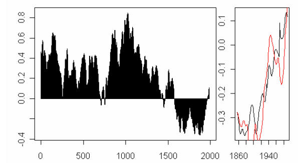
The Ababneh Sheep Mountain chronology only goes back to the mid-12th century. In order to assess the impact of the update on the Mann and Jones 2003 PC1, I spliced the Ababneh chronology post 1121 with the Graybill chronology prior to 1121 (and the two are within a good enough synch at that time to justify the splice for a first-cut analysis.) I then calculated a PC1 using the correlation matrix (not the Mannian method) and obtained the following PC1 (using the 6 sites in the Mann and Jones 2003 network).

mann_j27.gif
Figure 2. PC1s from the Mann and Jones 2003 AD200 Network.

The weights in this calculation are far more balanced than in the original MBH calculation. I note that I’ve been able to replicate the Mann and Jones 2003 PC1 to five 9s accuracy (prior to Mann splicing it) so I’m 100% certain that we’re talking apples and apples in terms of network.

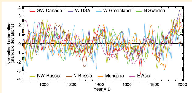
The Mann and Jones 2003 PC1 was not merely an important contributor to the very small Mann and Jones 2003 network, but was used in the (also small) Osborn and Briffa 2006 and Hegerl et al 2006 networks and even illustrated in IPCC AR4 as shown below (see the uptrending “W USA” series.
mann_j69.jpg

I’ll look at its effect on the MBH99 PC1 at some point, although this assessment is complicated by the fact the MBH AD1000 is still dominated by Graybill chronologies, most of which haven’t been updated, and the ones that have (San Francisco Peaks, Pearl Peak) haven’t been archived. Given the profound impact of using the Ababneh data on the Mann and Jones 2003 PC1, one does wonder even more at the failure of her colleague and thesis reviewer (Hughes) to use this updated data in Salzer and Hughes 2006, where he used Sheep Mountain in the now obsolete Graybill version.

Reference: Ababneh, L (2006). Ph.D Thesis, University of Arizona http://www.geo.arizona.edu/Antevs/Theses/AbabnehDissertation.pdf

Mann's co2detrend.f Calculation

Previous post (link).  A follow-up post (link)

If someone felt that it was necessary to detrend the bristlecone pine-based PC1 of Mann’s AD1000 network for CO2 fertilization, it’s doubtful that the initial instinct would be to coerce the data to a network of northern Canadian-Alaskan tree ring chronologies where the possibility of regional differences must surely be allowed for.

Inspection of Mann’s former FTP archive at the University of Virginia (which I fortunately archived before it was deleted) contains an interesting program entitled co2detrend.f (Mann’s main programs were not on the archive, but some programs were inadvertently left in the archive, including the program that calculated the tree ring network principal components – which was how we discovered Mann’s erroneous PC method.)

The program (which I’ve posted here) include the following interesting comments (in which Mann reports a correlation of 0.9 between the AD1000 PC1 and CO2:

c regress out co2-correlated trend (r=0.9 w/ co2)
c after 1800 from pc1 of ITRDB data

c remove co2-correlated portion (r=0.9) of 1800-1980
c
corr= 0.9

The program itself is in Fortran, which is highly verbose for simple operations like calculating a mean or standard deviation, that’s for sure. Below I’ve shown what is more or less a transliteration of his program into R so that you can see what the calculation does in simpler terms.

He first reads in the AD1000 Mannomatic PC1 and CO2 levels (with the 1610-1995 mean subtracted). I’ve uploaded both the source files to CA so that the commands below are fully operational (up to the need to take care with what WordPress does to quotation marks.) (The short R-script is here in ASCII form.)

First read in the data and make them into time series:

ser26= read.table(“http://data.climateaudit.org/data/mbh99/COMPARE/pc01.out”) # mannomatic pc1 1000-1980
ser26=ts(ser26[,2:ncol(ser26)],start=ser26[1,1])
ser12= read.table(“http://data.climateaudit.org/data/mbh99/COMPARE/ghg-lowf.dat”) # CO2 values less 1610-1995 average
ser12=ts(ser12[,2],start=1610) #this is the starting date based on other info

Then standardize the two series on the period 1800-1980 (as in the Mann program). inverting the PC1:

pc1= -ser26; #invert orienation
m1=mean(pc1[(1800:1980)-999]);sd1=sd(pc1[(1800:1980)-999]); c(m1,sd1) #[1] -0.01463 0.01858
standard1= (pc1-m1)/sd1 #1000 1980

m2=mean(co2[(1800:1980)-1609]);sd2=sd(co2[(1800:1980)-1609]); c(m2,sd2) #[1] 7.219 14.059
standard2= (co2-m2)/sd2 #1610 1980

Then subtract the CO2-adjustment from the Mannomatic PC1. The code in Mann’s program is (asum1 is the mean):

newpc1(i)=sd1*(standard1(i)-corr*standard2(i))+asum1

I implemented this as:

newpc=pc1; corr=.9
newpc[(1610:1980)-999]=sd1*( standard1[(1610:1980)-999]- corr*standard2) + m1

For the portion before 1610, I used the average CO2 value for the period 1610-1980 in the adjustment. Then plot. Here I’ve plotted the output from the co2detrend.f program against the “fixed” PC1 (which ties in to MBH99 Figure 1), both rescaled to match the scale of MBH99 Figure 1a.

coerci68.gif

The MBH99 CO2 "Adjustment"

We’ve all had enough experience with the merry adjusters to know that just because someone “adjusts” something doesn’t necessarily mean that the adjustment makes sense. A lot of the time, the adjuster arm waves through the documentation and justification of the adjustment. Today I’m going to work through aspects of one of the most problematic adjustments in this field: the MBH99 adjustment for CO2 fertilization – something that some of us have wondered about for a couple of years. In this particular case, there are a number of crossword puzzles and I’d welcome solutions to these puzzles, as I’ve pondered most of these issues for a long time and remain stumped. I’m not discussing here whether CO2 fertilization exists or not, but merely whether the Mannian approach is a reasonable approach to the issue, trying first merely to understand what the approach is.

I’m working towards assessing the impact of the new Abaneh Sheep Mountain data on the Mannian-style results – and the impact on the Mann and Jones 2003 PC1 (used by Osborn and Briffa 2006; IPCC AR4; etc.) Continue reading