The Ababneh Thesis

As I mentioned yesterday, Malcolm Hughes and/or the University of Arizona Laboratory for Tree-Ring Research had gone to the trouble of blocking my IP address from accessing their website. Thanks to the help of a couple of CA readers, I was able to circumvent the block. This is the sort of petty behavior that gives (or should give) the Team a bad name in a couple of senses – it both makes them look bad and it’s pointless because it’s readily circumvented. Given the relative ease of circumvention, you’d think that they wouldn’t bother, but they don’t seem to care. One CA reader wrote and asked me if he could locate what I was looking for. Originally I was just going to check their listserv, which I did, and there was nothing new there. But since I’d been blocked, I went to a little extra trouble to check the site and it was worth it. Continue reading →

Sargasso Sea dO18

Recently Keigwin’s Sargasso Sea dO18 temperature reconstructions have been mentioned in the climate public eye. Keigwin’s reconstruction famously has a warm MWP as shown below. This reconstruction uses modern dO18 measurements at Station S to calibrate two cores (with modern Station S values specifically shown in the graphic below):

I observed last year that the Juckesian version of the Moberg reconstruction had a very different appearance using Sargasso Sea instead of Arabian Sea G Bulloides and using Indigirka instead of Yamal – a point that I re-iterated recently in light of the final Juckes paper. I discussed Juckes and the Sargasso Sea last year and in my Review Comments at CPD. We’ve discussed the Juckesian pretext for withholding the results with Indigirka. His pretext for excluding the Sargasso Sea SST reconstruction from dO18 is that the data ends in 1925 (a point was recently picked up at realclimate).

The Sargasso Sea series used by MSH2005 is sometimes mistakenly presented as having a 1975 data point representing the 1950–2000 mean, but the actual end point is 1925 and so this series is also omitted.

Today I want to discuss exactly what is and isn’t in the Keigwin Sargasso Sea data, amending some first thoughts based on clarifications provided below by several readers. Keigwin (1996) (see here) archived a data set with SST, salinity and dO!8 values from 1955 to 1995 here . Keigwin 1996 says:

As expected, the effects of decreased SST and increased salinity during the late 1960s combined to increase the dO18 value of equilibrium calcite. Over the full 42-year series, linear regressions between the SST, salinity and dO18 values show that temperature accounts for about two-thirds of the isotopic signal ( r2 = 0.61), whereas salinity accounts for one-third (r2 = 0.29). Thus, by comparison to sea surface changes during the past several decades, it is reasonable to interpret the foraminiferal isotopic data mostly in terms of SST change.

This statement, combined with the data set, looks like a calibration set. The above discussion – in which variance is allocated to factors – looks very much like a conventional statistical analysis. As I observed in my first cut at this:

The statistical model from the two-factor model is so uncannily accurate (r2= 0.9988) that I’m wondering whether some of the data here has been forced somehow. Actual and fitted dO18 values are shown below: you have to look very closely to see any discrepancy. The dashed line is not simply a replot of the data: you can notice some very small differences. I’ve never seen any proxy model that is remotely this accurate – so it is puzzling. Some time, I’ll try to check whether (say) the salinity measurements are forced and that’s why the model is so accurate.

My surmise that the model was forced was correct, but I missed what was being forced. The explanation is latent in the article – it’s just that what was being done was something that I hadn’t expected. Keigwin forced the dO18 values from SST and salinity measurements at Station S and then did a regression using the forced data set.

In order to gauge the influence of the annual variability of SST and salinity on the oxygen isotope ratios that might be recorded by surface-dwelling foraminifera at Station “S”, I calculated the 6% value of calcite precipitated in oxygen isotopic equilibrium with seawater (Fig. 3) (26).

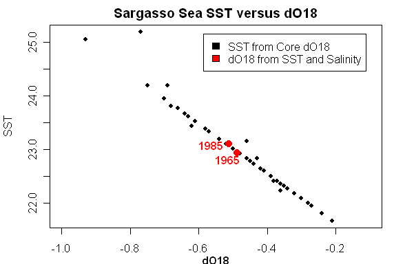
What exactly does this calculation do – I guess that it somewhat quantifies the expected contributions of salinity and SST to dO18 variation, given the measured variability of SST and dO18. Here’s a way of representing the calculation which clarifies things for me: the black points show reconstructed SST from core sediments against the dO18 of the core sediments (in a linear relationship according to the reconstruction transfer model), while the red points show two 20-year averages of reconstructed (“modeled”) dO18 from measured SST and salinity using the Deuser/Keigwin methodology. Keigwin observed that core dO18 values (which integrated decadal periods) were outside the range of modern (estimated) values from Station S using current transfer models. His plot shown above amalgamates the modern and core data along these lines.

sargas22.gif

While I was looking at this data, I became intrigued with some of the properties of the original calibration of dO18 to SST in the Station S data set, which illustrate rather nicely some of the issues involved in reconstructions of any kind. The dO18 values here are forced and that’s why the model is 100% accurate. But let’s suppose that we actually did have a 100% accurate model and see what the effect of not knowing salinity does to the error structure of SST reconstructions. These are just thoughts right now.

Two-Factor dO18 Model
Although dO18 is used to reconstruct SST, the actual physical relationship goes from SST and salinity to dO18. As an experiment, I tried a simple regression of dO18 values against SST and salinity data as follows:

fm=lm(dO18~SST+Sal_psu,data=sarg.mod)

sargas16.gif

First, let’s look at the dO18 model (note that we’re fitting dO18 here rather than SST) if we just use SST for the reconstruction, as shown below. You can readily see that the model using only SST is less successful and that the residuals from the model leaving out a factor have positive autocorrelation (and a failed Durbin-Watson statistic.) This is a rather nice demonstration of how the Durbin Watson statistic gives evidence that a salient factor has been left out of the model. In econometrics, this is evidence that the model is mis-specified – a statistical method that Juckes et al for example simply repudiated without providing any statistical authority. Juckes’ say-so was high enough authority for editor Goosse, I guess. In this case, there is a fair amount of autocorrelation in the salinity data and this carries forward into the residuals from the incompletely specified model.

sargas18.gif

The above plot illustrates the situation for the modeling of dO18. However in climate studies, the procedure of interest is the reverse: the use of dO18 as a “proxy” to “reconstruct” SST. A common strategy is the use of “inverse regression” of SST against dO18 -even though the physical relationship is the opposite. I use the term “inverse regression” here as it’s used in calibration statistics off the Island. There’s been much made of inverse regression in climate science (von Storch, Juckes), where the term “inverse regression” does not coincide with “inverse regression” as used in conventional statistics, but to describe a variant of partial least squares used on the Island in various guises- a topic that I’ve discussed here. If the calibration is done from the regression of dO18 against SST, this is called “classic calibration” in calibration studies. For the discussion here, don’t worry about the terminology in the various studies, but about what is being done. Here I’m regressing SST against dO18 as shown below:

fm.inv=lm(SST~dO18,data=sarg.mod)

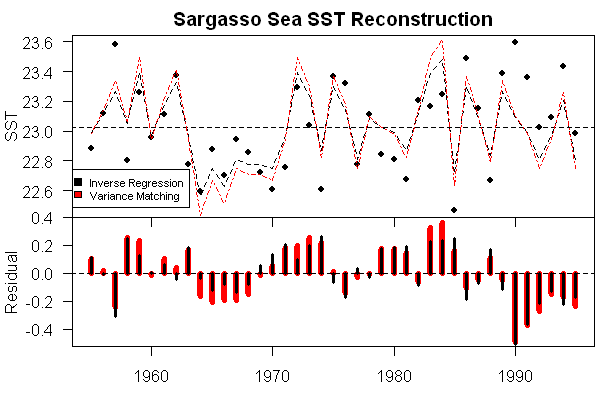
The figure below shows the SST reconstruction (top) and residuals (bottom) using inverse regression based only on SST – a defective model to be sure, but a model containing some information. I’ve also shown the reconstruction using variance matching. In a univariate case, this simply dilates the reconstruction a little, in which the price for matching the variance is the increase in the average size of the residuals. As you can readily see, the autocorrelation in the reconstruction residuals is intimately related to the defective model (in which the autocorrelation of the salinity is imposed onto the residuals.) You can also see that the variance-matching reconstruction and the inverse regression reconstruction are intimately related, with the one just being a dilation of the other.

sargas19.gif

Thus, estimating the confidence interval of the reconstruction depends on the size of the impact of unreconstructed salinity. Because the mis-specified factor has considerable autocorrelation, the confidence intervals cannot be calculated in an elementary way. A common recipe in climate studies is to estimate the reduction in number of degrees of freedom. While the approach is not absurd, the devil is always in the details. I think that the salient question is: how many measurements are needed in an average so that the probability of the average error being within \epsilon of 0 corresponds to a “standard” value using i.i.d. normal errors. Some time, I’ll re-examine the typical recipes on the Island.

It should also be a little sobering to see how large the errors are in this case when one factor is unavailable for a proxy where, in this case, due to forcing, the model is specified to 100% accuracy. The standard deviation of the residuals was 0.2, while the standard deviation of the SST was 0.29 – this is in a perfect model with unknown salinity. If the dO18 model explained (say) 50% of the variance in the model, then these errors would have to be added in. I’ll do the calculations some time to try to figure out where the model “breaks even”.

USHCN #3

Unthreaded #22

Almagre Vistas

I hope that many of you have visited Pete Holzmann’s photo gallery here. If you click on each picture on this page, you get a separate “gallery”. Today, I’m going to post up a quick overview together with a few maps. Continue reading →

A Little Secret

Don’t you think that someone on the Team might have been a little curious as to what bristlecone ring widths have done during the past 25 years? For this, we have the classic excuse of Michael Mann and the Team for not updating bristlecone and proxy records is that it’s not practical within the limited climate budgets:

While paleoclimatologists are attempting to update many important proxy records to the present, this is a costly, and labor-intensive activity, often requiring expensive field campaigns that involve traveling with heavy equipment to difficult-to-reach locations (such as high-elevation or remote polar sites). For historical reasons, many of the important records were obtained in the 1970s and 1980s and have yet to be updated.

From the first moment that I got involved with paleoclimate, it seemed obvious to me (as it is to anyone not on the Team) that, if the classic “proxies” are any good and not merely opportunistic correlations, that there is an ideal opportunity to perform out-of-sample testing of the canonical Team reconstructions by bringing the proxies up-to-date. I wrote an Op Ed in February 2005 for the National Post entitled “Bring the Proxies Up to Date”, where I expressed the view that this was really the first order of business in Team world. While the addition of new proxies is also important and nice, this is not the same thing as out-of-sample testing of the proxies used in MBH99, Crowley and Lowery etc – especially the bristlecones.

I’ve continued to satirize this failure pointing out that several of Graybill’s classic bristlecone sites were easily accessible from UCAR world headquarters in Boulder and that no heroic expedition was required to update, for example, the Graybill sites to the west of Colorado Springs.

To get to these sites from UCAR headquarters in Boulder, a scientist would not merely have to go 15 miles SW of Colorado Springs and go at least several miles along a road where they would have to be on guard for hikers and beware of scenic views, they would, in addition, have to go all the way from Boulder to Colorado Springs. While lattes would doubtless be available to UCAR scientists in Colorado Springs, special arrangements would be required for latte service at Frosty Park, though perhaps a local outfitting company would be equal to the challenge. Clearly updating these proxies is only for the brave of heart and would require a massive expansion of present paleoclimate budgets. No wonder paleoclimate scientists have been unable to update these records since Graybill’s heroic expedition in 1983.

Pete Holzmann (Mr Pete), who lives in Colorado Springs, agreed with this satire and this led to what I’ll call the Starbucks Hypothesis: could a climate scientist have a Starbucks in the morning, collect tree rings through the day and still be home for dinner?

To make a long story short, last summer, when my wife and I visited my sister in Colorado Springs and I thought that it would be rather fun to test the Starbucks Hypothesis and I gave a bit of a teaser report in late July, promising some further reports in a few weeks, but I got distracted by the Hansen stuff. At the time, I mentioned that, together with CA reader Pete Holzmann and his wife Leslie, we visited some bristlecones in the Mt Almagre area west of Colorado Springs.

But I have a little secret which I’ll share with you as long as you promise not to tell anyone: our objective was to locate the precise site sampled by Graybill. Not just that. Prior to the trip, I obtained a permit from the U.S. Forest Service to take dendrochronological samples from bristlecones on Mount Almagre and we did more than look at pretty views; we obtained up-to-date bristlecone samples. I only went up Almagre on the first day. Our permit lasted a month and Pete and Leslie spent two more days on Almagre, finally locating and sampling tagged Graybill trees on the third day.

Altogether (and primarily through the efforts of Pete and Leslie), our project collected 64 cores from 36 different trees at 5 different locations on Mount Almagre. 17 Graybill trees were identified, of which 8 were re-sampled. All the cores are currently at a dendrochronological laboratory, where sample preparation and scanning steps have been completed. Cross-dating is now taking place. For the most part, we tried to sample non-stripbark trees in keeping with NRC recommendations, but some stripbarks were sampled to reconcile with Graybill. Of the tagged Graybill trees, the tag numbers do not reconcile with the archive identification numbers and, in the absence of any concordance, reconciliation may prove more difficult than one would think.

We will archive at WDCP detailed information on the location of all samples (current spreadsheet is here) , which has already been sent to the U.S. Forest Service. Photographs of each tree are shown gallery here. Here’s a fun presentation that Pete prepared of our Day 1 itinerary. Here is a Google Earth tour. If you run it and when Google Earth comes up, go to Tools “ Play Tour , you’ll have some fun.

Some expenses have been incurred for this expedition. Leaving aside travel expenses (which were vacation expenses that I was going to incur anyway), the jeep got a bad scratch on the first day and cost about $500 to repair plus some more repairs from Days 2 and 3; it’s going to cost a few thousand at the dendrochronology laboratory for the sample prep, scanning and cross-dating as this has been done on a contract basis. I’ve submitted an abstract to Rob Wilson’s divergence session at AGU and would like to present these results (and to cover Pete’s expenses if he can come). On the basis that we submit a data paper to a journal, publication expenses will be another $800-1000 or so (academic authors pay the journals to publish). This has been a Climate Audit project so I’d like readers who contribute to the top jar to think about a special contribution for the bristlecone sampling. Maybe Martin Juckes, James Hansen and Michael Mann will contribute as well – I’m sure that they are all anxious for the results.

I’ll add some more information later in the day. Right now I’m off to visit the dendro lab and see how things are coming along. In 2002, Malcolm Hughes sampled bristlecones at Sheep Mountain and nothing has been reported or archived from this study. In 2003, Lonnie Thompson sampled ice cores at Bona-Churchill and we’ve heard nothing about it. One might guess that 20th century dO18 levels were not high as, at the nearby site of Mount Logan, 20th century dO18 levels were lower than earlier levels, attributed to regional changes in circulation rather than temperature.

I’ve obviously been very critical of what appears to be opportunistic reporting of results. With my experience in mining speculations, I fully understand how much temptation that there is to delay reporting of “bad” results in the hope that later drill holes in the program will salvage things. But you don’t have any choice in the matter – you’re obliged to report the results. Plus investors are smart enough to now that delayed results are virtually never good results.

Right now I have no idea what the sampling will show – maybe it will show a tremendous response by the bristlecones in the past 20 years – perhaps due to CO2, nitrate or phosphate fertilization, perhaps due to temperature increases. Maybe they won’t go up and we’ll hear more about the divergence problem. I don’t expect these particular measurements to settle anything. But jeez, doncha think that someone would have tried to find out?

Anyway I promise one thing: the measurements are going to be made public as soon as I get them. Just like a mining project. No waiting for 5 or 10 or 25 years like certain people. No losing the data like other people. Whatever they show. As soon as I get the cross-dated measurement data, we will immediately send it to the World Data Center for Paleoclimatology (which I expect to take place within a few weeks.) I hope that this will set an example to the trade as to the type of turn-time which is practical.

I’m visiting the dendro lab today to say hello and I wanted this to be on the record before my visit. I’m not sure how far along they are, but I think that they’ve finished sample prep and scanning and have started cross-dating. I don’t expect any results, but they may be far along enough so that I’ll have an impression of what the result growth will have been. So I wanted to be on the record on the planned schedule prior to my knowing anything about the results, just in case I get an impression today of what the recent growth has been.

UPDATE 2 pm. OK, I’m back from the dendro lab in Guelph. They are further along than I expected. The longest core is 883 years (Tree 30A). This had a Graybill tag 84-55, but if you go to the archived measurement data
and look for ALM55 (which would presumably be the match), there are no corresponding measurements; there is obviously a sequence ALM01, ….; there is an ALM53 and an ALM60. Is there an alter ego somewhere or is it missing? Right now we don’t know.

After sanding the core is scanned. The measurement of ring widths is semi-automatic. For these bristlecones, earlywood and latewood was easy to distinguish. Using a magnified version of the scan, each ring is picked out (with the computer recording the pick). The computer then yields back the measurements. I’ve posted up a couple of print-screens showing the most recent widths for 30A and the widths in the mid-19th century.
.

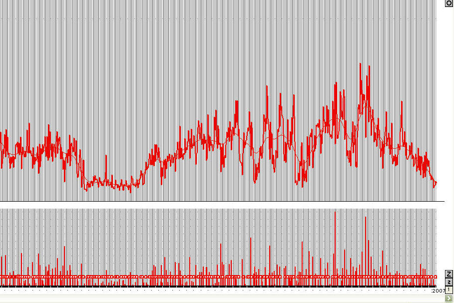
Below is a print screen showing the 30A ring widths from 1124 to 2007. I’ll post up a re-plot at some point with a legible x-axis. For orientation in the absence of a scale, the upspike on the left is 1174; there are low values from 1353 through the early 1400s; there is a 1690 spike; 1865 and 1880 are upspikes; 1941 is a small upspike.

According to the Team hypothesis of a positive linear relationship between temperature and ring widths, the warm 1990s and 2000s should have yielded the widest ring widths in history. What do you think? This is only one tree, but my quick impression was that recent growth was not elevated. So this looks like a Divergence “Problem”. If CO2 or other fertilization has been a factor, then I hate to think what the growth would have been without the fertilization. Remember the NAS panel saying that the Divergence Problem only affected high-latitude sites? Maybe they should have done some testing before they opined on this.

BTW while I’m critical of how the Team uses dendro information, I think that it is well worth supporting the collection of dendro information, even if it’s meaning is not clear right now. It has the advantage of being well-dated – and when you see the problems with dating ocean sediments, it’s nice to have some records that are well dated. There’s a role for it; so please – no posts dumping on dendrochronology. The dendrochronologists who’ve been doing this work (and who I will credit in due course) are excellent people.
almagr8.jpg

Tree 30A Ring widths. 2007 on right. i’ll replot this some time soon. For orientation in the absence of a scale, the start is 1124; the upspike on the left is 1174; there are low values from 1353 through the early 1400s; there is a 1690 spike; 1865 and 1880 are upspikes; 1941 is a small upspike.

Juckes and the West Greenland Stack

Last fall, I discussed information sources on West Greenland ice core series, noting that the West Greenland version attributed by Juckes to Jones et al 1998 was a version that I’d not seen before. While I was looking at the proxy decisions in Juckes et al, I noticed the following intriguing rationalization:

The Greenland stack data used by MBH1999 is a composite of data analysed by Fisher et al. (1996), but the precise nature of the composite is not described by Fisher et al. (1996). … The Crete ice core series [of Jones et al 1998] is preferred to the “stack” series used by MBH1999 because it is better documented.

So one asks: exactly what is the “better documentation” preferred by Juckes and the Euro Team? Or is this “better documentation” a figment of their imaginations?

Jones et al 1998 and MBH98-99 both cite Fisher et al 1996 as a reference. As it happens, Fisher et al 1996 does not appear to describe either series (it only illustrates rather short versions, although it describes Fisher’s stacking methodology.) So any documentation advantage in this reference is a draw.

Fisher (2002) Table 1 reports the use of a version identified as DELNORM6.CWG (with that exact nomenclature) – “CWG” standing for Central West Greenland.: the file itself was ASCII. A couple of years ago, Fisher sent me a CD with a variety of series on it. Experimenting a little, I determined that the series DELNORM6.CWG, included on the CD, matched the MBH99 version 100%. The DELNORM6.CWG file listed its components for each step e.g. the following components in one of the steps. So any person who received the DELNORM6.CWG version from Fisher would have received a relatively adequate recipe for how it was constructed. In Mann’s MBH98 data archive, the email transmitting this series to Mann (from Frank Keimig of the University of Massachusetts) is preserved for some reason.

A CT85A-1Y.CRT 1983 AD 362 212 144
B CT84B-1Y.CRT 1982 267 211 50
D CT84D-1Y.CRT 1982 217 211 0
CRETE CT74-1YS.CRT 1973 922 202 714
MILCT MC73-1Y.MIL 1966 791 195 590
GISP2 GISP1YR.GSP 1985 718 214 498 DEUTERIUM
GRIP SIG#1YR1.GRIP 1979 917 208 703
GRIP SIG#2YR1.GRP 1979 917 208 703
GRIP SIG#3YR1.GRP 1979 917 208 703

I’ve attempted to locate the Jones et al version within the many variations in Fisher’s files, but so far have been unable to locate an exact reference. There are multiple series from Crete, including many of the series in the Fisher stack described above (Crete, A, B, C, D, H). The Jones version is not the same as any of the potential components. The Jones version goes from 1000 to 1983; the only version going back to 1000 (actually to 553) ends in 1973; there are a number of potential components ending in 1983, but all start after 1000. So the Jones version appears with a high degree of probability to also be a CWG stack – except in this case, unlike DELNORM6.CWG, we don’t know the precise components of the stack, although the Jones version is obviously closely related to these components.

So back to the question: is the “better documentation” of the Jones version a figment of the Euro Team’s imagination – the full team including Briffa, Osborn, Moberg, Allen, Hegerl, Weber, Esper. It sure seems that way to me. Perhaps Juckes can identify some such documentation, but he didn’t do so in the article itself. I guess Goosse and the referees didn’t ask him about it.

In addition, given Juckes’ professed concern about ensuring that all series versions have properly received permissions from their originators, it’s interesting to contemplate what permission (if any) Juckes has for archiving the Jones et al version of the Fisher data (or for that matter the MBH version.) I am unaware of any public archiving of either version by Fisher himself.

I presume that Frank Keimig got the DELNORM6.CWG version from Fisher either directly or indirectly. In the email at Mann’s FTP site, Keimig mentions re-formatting the series – in which process the documentation in the Fisher version was removed. Mann got this version from Keimig; Juckes presumably got it from Mann, either directly or from Mann’s archive. Did anyone in this chain ever get permission from Fisher to archive the data publicly? I doubt it. I don’t suppose that Fisher has any objections to people using his data provided they acknowledge him – why would he? But within Moberg’s definition, Fisher himself, to my knowledge, never publicly archived the version now disseminated by Juckes.

I believe that the Jones version is an earlier version of the DELNORM6.CWG series (or some close variation.) Jones may have got his version directly from Fisher who’s very cooperative (or he could have got it from Ed Cook or someone like that indirectly). Presumably Juckes got the Jones version from Briffa or Jones. (BTW Jones refused to provide the versions that he used to me when I requested.) Moberg expressed concern about the possibility of Sidorova issuing a new version and that he did not want to preempt any adjustments by Sidorova to her series. It seems inescapable that the DELNOM6.CWG version (which is used in Fisher 2002) is a version that Fisher prefers to the version used in Jones et al 1998. Yet Juckes seems to have no compunction about not only archiving the Fisher version used in Jones et al 1998 version – a version that never previously had been posted on the internet digitally – and in using a version seemingly not preferred by the originator of the data, all using the pretext of “better documentation”, though no evidence of such “better documentation” was provided anywhere.

References:
David A. Fisher, 2002. High-resolution multiproxy climatic records from ice cores, tree-rings, corals and documentary sources using eigenvector techniques and maps: assessment of recovered signal and errors, The Holocene 12,4 (2002) pp. 401-419
Fisher, D. A., Koerner, R. M., Kuivinen, K., Clausen, H. B., Johnsen, S. J., Steffensen, J. P., Gundestrup, N., and Hammer, C. U.: Inter-comparison of ice core and precipitation records from sites in Canada and Greenland over the last 3500 years and over the last few centuries in detail using EOF techniques, NATO ASI Ser, Ser. I, vol. 41, edited by: Jones, P. D., Bradley, R. S., and Jouzel, J., pp. 297–328, Springer-Verlag, New York, 1996.

Juckes and "Restricted" Data

Many climateaudit readers will remember Mann’s “CENSORED” directory, in which Mann calculated principal components on a network that excluded bristlecone pines (which needless to say didn’t have a HS shape. Now Juckes et al introduces us to a new type of climate data: “restricted” data. The Team has introduced a novel data classification system – PG and R. Juckes et al say that the Indigirka series is R-rated and so it can’t be used in their reconstruction. Yes, R-rated tree ring data. Data so salacious that you have to keep it under lock and key.

Is it only under-18s that are not allowed to see R-rated tree ring data? Can we show it here if Kristen Byrnes promises not to look?
Or are all climateaudit readers prohibited? Is this a bit like pornography that is only available to priests? You think that I am juck-ing? Here are their exact words from the Euro Hockey Team for excluding the Indigirka series:

The Indigirka series used by MSH2005 is not used here because it is not available for unrestricted use.

I wonder what went through the minds of editor Goosse when he read that this was a “restricted use” proxy? Did Goosse ask what the restrictions were? Or referee Gerd Bürger or the other two anonymous referees? Since they don’t appear to have asked or weren’t bothered by the answer, let’s ask the question here. And, by the way, for readers who may be offended by salacious tree ring data, proceed at your own risk as the R-rated data is shown graphically in the post continuation. Yes, you too can see what the climate priests keep in their secret cupboard. If you are not over 18, please do not continue without parental guidance. Continue reading →

Gridding from CRN1-2

In order to assess the 2006 anomaly in John V’s 2006 calculation reported previously, I’ve calculated a gridded anomaly for the U.S. using standard spatial smoothing software in R. This enables the calculation to be done in a few lines as explained below. I’ll also show results which reconcile most of the results to date. I’ve shown the details of calculation step so that there will be no confusion. I also want to show how simple it is to produce gridded data from station data. It only takes a couple of lines of code.

CRN Ratings
First I downloaded the current ratings from Anthony Watts from http://www.surfacestations.org/downloads/USHCN_stationlist.xls and saved it as a tab-separated ASCII file. I first deleted the comment columns and changed the apostrophes to _. This is important for R programs. I then added these ratings to my USHCN info file details as follows:

url=”d:/climate/data/station/watts”
#downloaded from http://www.surfacestations.org/downloads/USHCN_stationlist.xls
#some columns deletedl also replace ‘ with _
loc=file.path(url, “stationlist.txt”)
watts=read.table(loc,sep=”\t”,fill=TRUE,nrow=1221,header=TRUE)
details$watts=NA
test=match(details$id,watts[,”USHCN.ID”]);temp=!is.na(test); sum(temp) #1221
details$watts[temp]=watts[ test[temp],5]
details$watts[(details$watts==0)&!is.na(details$watts)]=NA

I then loaded my collation of USHCN station data and extracted the stations with CRN ratings of 1 or 2 as follows:

load(“d:/climate/data/station/ushcn/ushcn.collation.tab”)
temp=(details$watts< =2)&!is.na(details$watts);sum(temp)
index_good=(1:1221)[temp]
good=ushcn.collation[[2]][,index_good] #2544 53
M=ncol(good)

Anomaly Calculation
I then converted this to an anomaly basis and calculated annual averages. I did a separate calculation for 2006 using available months only. The functions anom and ts.annavg are available in scripts/gridcell/collation.functions.txt.

good.anom=good
for(i in 1:M) good.anom[,i]=anom(good[,i])
good.ann=ts( array(NA,dim=c(nrow(good)/12,M)),start=tsp(good)[1])
for(i in 1:M){ good.ann[,i]=ts.annavg(good.anom[,i])}
temp=(c(time(good.ann))>=1890)
good.ann=ts(good.ann[temp,],start=1890)
time0=c(time(good.ann)) #1890:2006
for(i in 1:M) good.ann[N,i]=mean(good.anom[(nrow(good.anom)-11):nrow(good.anom),i],na.rm=T)

Gridding
Gridding is a type of spatial smoothing for which there are a variety of standard functions and no need for people to ponder over triangles or hexagons (which don’t matter much) or to write new code. If one wants to vary smoothing parameters (in this perspective, GISS smooths much more than CRU), then one should do so in the context of standard software where there is working experience. In this case, I used the function interp from the R-package akima (which I had previously installed.) I used three “masks” to screen out values which otherwise would get interpolated into the ocean or into Canada (tho not much turns on this.) Because each gridpoint represents an equal area, I simply calculated the mean of the values.

library(akima)
N=length(time0)
annual=rep(NA,N)
for (j in 1:N){
X=data.frame(details[index_good,c(“long”,”lat”)],good.ann[j,]) #locations of “good” stations
names(X)=c(“long”,”lat”,”anom”)
temp=!is.na(X$anom)
gridded < – interp(X$long[temp], X$lat[temp], X$anom[temp])
gridded$z=gulfmask(gridded$z)
gridded$z=atlmask(gridded$z)
gridded$z=canadamask(gridded$z)
annual[j]=mean(gridded$z,na.rm=T)
}
annual.tobs=ts(annual,start=1890)

The mask functions were not particularly elegant. The akima package with this data yields a 40×40 grid and I simply set values at inappropriate gridpoints to NA as follows.

gulfmask=function(Z){
Z[21:31,1:2]=NA;Z[21:30,3]=NA;Z[22:30,4]=NA;
Z[23:30,5]=NA;Z[c(23:24,27:30),6]=NA; Z[27:28,7]=NA; Z}

atlmask=function(Z){
Z[40,c(1:26,29:31)]=NA; Z[38:39,1:26]=NA; Z[37,1:23]=NA;
Z[36,1:16]=NA;Z[35,1:15]=NA; Z[34,1:13]=NA;Z[33,1:11]=NA;
Z}

canadamask=function(Z){
Z[40,37:40]=NA; Z[37:39,35:40]=NA; Z[36,34:40]=NA;
Z[34:35,32:40]=NA;Z[32:33,29:40]=NA; Z[31,c(28:29,33:40)]=NA;
Z[30,36:40]=NA;Z}

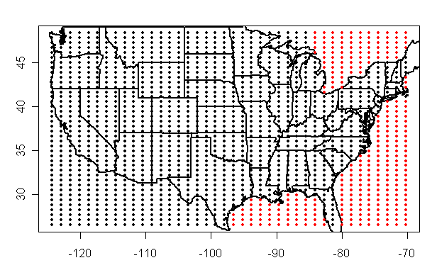
Here’s an illustration of the points that are masked out by these masks. I didn’t bother with masks in other places because the algorithm didn’t interpolate over there, but it could be esily done.

usgrid52.gif

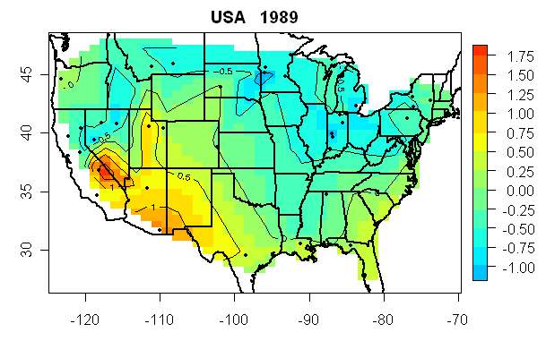
Here’s an example of the type of annual map that is generated by the smoothing function. This was generated by doing a single step and plotting from the object gridded produced in the above routine as follows (using the R package fields). You’ll note that this smoothing function does not calculate gridded values at the edges which are an extrapolation from the stations. (This map also shows the stations used in the calculation.)

par(mar=c(3,3,2,1))
breaks0=seq(-3,3,.25)
image.plot (gridded$x,gridded$y,gridded$z, col=tim.colors(length(breaks0)-1),breaks=breaks0,ylab=””)
contour(gridded, add=TRUE,ylab=””)
points (X$long[temp],X$lat[temp], pch = 19,cex=.7)
US(add=TRUE,lwd=2)
title(main=paste(“USA “, time0[j]))

usgrid53.gif

So it’s pretty easy to do a gridding calculation using standard software. Hansen’s program has very ad hoc statistical methods in which stations are adjusted from other stations and gridcells calculated. At the end of the day, the best approach to this aspect of his program will probably be to see what smoothing parameter best emulates his method and thereby restore it to a known statistical methodology.

COMPARISONS

First here is a comparison of my calculation using CRN1-2 data to NOAA results from 1890-2007. (I re-iterate for the N-th time that analyses on U.S. data are not representative of the ROW.) NOAA has values to Aug 2007 and I’ve estimated the last 4 months as the same as the corresponding 2006 months for now. NOAA has run warmer by about 0.2 deg for the past decade and was about 0.1 deg C cooler in the 1930s.

usgrid54.gif

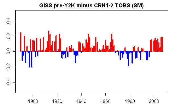
Second here is a comparison of CRN1-2 data to GISS pre-Y2K results. As you see the GISS with the Y2K error was running warm by about the same as NOAA – which may be one reason why they didn’t spot the error. GISS runs a bit warmer than NOAA in the early and mid portions of the graph due to their greater efforts to do an urban adjustment.

usgrid55.gif

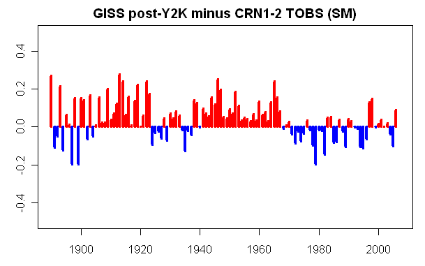
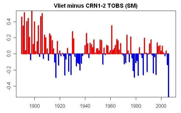
Third, here is a comparison of CRN1-2 data to GISS post-Y2K results (but not including the September change from SHAP to FILNET, which seems much too opportunistic.) Relative to CRN1-2, GISS tends to warm the cool periods (1960s, 1900s) and to cool the warm periods (1930s), reducing the size of the mid-20th century cooling. For the U.S., as noted before, by using the trends from “unlit” stations to establish trends – in a context where there are a lot of decent rural stations with long records – the GISS methodology for USHCN stations seems more appropriate than the NOAA (and probably the CRU methods). Unfortunately, this method is not used in the ROW, where there is nothing equivalent to the USHCN.

usgrid56.gif

Finally, here is a reconciliation to John V’s annual results sent ot me yesterday. His 2006 results run much colder than the ones that I calculate- which is presumably an artifact of the 3 months stub period that he used in his calculation. So the anomaly with his 2006 results can be traced definitely to this (which shows up a “cool” difference in the graph below.)

usgrid57.gif

So what does my calculation using CRN1-2 data look like: see below, which includes a 2007 estimate (using the 2006 difference between the CRN1-2 and NOAA to estimate 2007 CRN1-2 from the YTD NOAA results.) In this calculation, the warmest year remains 1934 by a margin of nearly 0.2 (enough to be “statistically significant” according to things that GISS has said, then 1921, then 1998, then 2006 in fourth place. Values since 1998 have been at uninterrupted high levels. Looking at the graph, it’s definitely noticeable – but is it the sort of change that’s inconsistent with the sort of stochastic behavior in the early part of the series – hard to tell here. If you cut the series off in 1997, you certainly wouldn’t have noticed anything odd about the 1990s. You can sort of see in retrospect why MBH98-99 were so excited about how warm 1998 and in such a rush to include it in their article. The main verification issues right now is why the ROW history is so different from the US – is it climatic or nonclimatic? And can one tell?

usgrid58.gif

2006 and CRN1-2

John V has posted some graphics recently arguing that CRN1-2 yielded pretty much the same results as major temperature indices and, in some sense, vindicated these results. As Gavin Schmidt has pointed out, the U.S. is only 2% of the world’s surface; and as I’ve observed on many occasions, the statistical methodologies and data quality in the U.S. are different from the ROW, as is the history.

I’ve been focussing more on ROW issues recently rather than U.S. issues, but thought that it would be interesting to drop in briefly on the U.S. issues. Since there seems to be an interest in gridding, I’ll probably do a version, using the methods that I used to contour the trend maps a while ago. I also thought that it would be interesting to verify John V’s CRN1-2 estimate to NOAA and NASA versions myself.

I mention 2006 in the header because there’s something interesting about 2006 which hasn’t been mentioned in John V’s posts: 2006 values for both NOAA and NASA are as much as 0.8 deg C higher than CRN1-2 values.
Continue reading →