Something Fun from Sinan Unur

OK, so I got interested in decoding the binary data sets at ftp://data.giss.nasa.gov/pub/gistemp/download/ as well. Wrote some Perl to slice and dice the data set into various series. I now have fully 1.6Gb less free hard drive space and I cannot figure out where my Sunday went ๐Ÿ™‚

I’ll tidy up the various scripts and post on my web site when I get a chance. The result of my attempt at visualizing TSurf1200 and SSTHadR2 combined is available on Google Video.

Enjoy.

Sinan

Lovelock and the Revenge of Gaia

From Webster’s dictionary

Totem n

1. a natural object or an animate being, as an animal or bird, assumed as the emblem of a clan, family, or group.
2. an object or natural phenomenon with which a family or sib considers itself closely related.
3. a representation of such an object serving as the distinctive mark of the clan or group.
4. anything serving as a distinctive, often venerated, emblem or symbol.

It was William “Stoat” Connelley, Wikipedia administrator, keeper of multiple blogs, Green Party candidate and, one hopes, assiduous climate modeller during his spare time, who gave the reason why we keep encountering a certain statistical reconstruction of past climate in response to my query

Of course, the mere fact that the “totemizing” was propagated by the IPCC, the environmental lobby and especially the authors of this blog as “the scientific consensus” should cause disinterested viewers to wonder as to who is trying to fool who.

Stoat replied:

Response: in fact the totemising has mostly been done by the skeptics.

One of the doyennes of what can fairly be described as climate alarmism would be the author James Lovelock, creator of the suspiciously anthropomorphic Gaia Hypothesis. In 2006, Lovelock published his latest polemic on the state of the world: “The Revenge of Gaia” in which all sorts of catastrophes awaited the world, including the dread spectre of Global Warming.

In the section on global warming, which comes rather incongruously after a discussion about astronauts falling into black holes, Lovelock reveals his secret weapon:
Continue reading

Unthreaded #6

Continuation of Unthreaded #5

FOI Request to Phil Jones

Some feedback on my request for the sites used in Jones et al 1990 (no data): Continue reading

Juckes Reply #3

Juckes also replied to CA reader Mark Rostron and there were a couple of interesting aspects to the response.

1. In a Millenial reconstruction, it would be helpfull to know how many data points were
available for each measured time period over the thousand years. Fig 2 indicates that
the number in the early years may be quite small.

(1) Figure 2 refers to data used in the Mann et al. (1999) paper. In our reconstruction
we use only data which are available throughout the study period, 13 time series in the
revised manuscript.

2. How much recent data is there? Does the sampling end in 1980, 26 years ago?

(2) Many of the proxy series end in the 1980’s. For calibration purposes it is important
that proxies are from sites which have been undisturbed. This is now rather harder to
ensure because of the spread of agriculture and nitrogen pollution.

3 Although Climate Models are mentioned, there are no references to any climate
model that has accurately predicted temperature, are any available?

(3) There is a discussion in the IPCC report.

4 Appendix A2 says that “This method starts out from the hypothesis that different
proxies represent different parts of the globe”, but there are no correlations shown to
local temperature see Table 1 and 2. Has any test been done to see if the Proxies
correlate well with local temperatures. Is any local temperature data and correlation
available?

(4) Local correlations are only meaningful if the signal to noise ratio is greater than
unity. This is not the case here.

5 What is the justification for including low correlation proxies listed in Table 1?

(5) As above.

6 Although Table 2 shows a cross correlation between different data bases, there is no
cross correlation between individual proxies. Do the various Proxies correlate well with
each other in the non instrumental temperature period?

(6) Yes: Jones et al (1998) comment on this. We have looked at this, but have not
found any new results.

Here are a couple of points that caught my eye here. The original Juckes et al submission had 18 proxies; now they have 13 proxies. I wonder which proxies have been subtracted. I presume that the duplicate versions of Tornetrask have gone to one version, but who knows. There’s an amusing aspect to this. Juckes’ statistical model for CVM stated:

This method starts out from the hypothesis that different proxies represent different parts of the globe

This can obviously be said about anything. So Juckes et al used two Tornetrask versions – did these “represent different parts of the globe”? Maybe one Tornetrask series “represented” Sweden and the other Tornetrask series “represented” Antarctica or South Africa. Anything is possible in their model as stated. Alternatively, if one wanted to test the hypothesis that the Juckes proxies represented different parts of the globe, one way of testing the hypothesis would be to plot the locations. Now Juckes had multiple different geographical locations for Tornetrask, including the middle of the Baltic Sea, but I think that he’s prepared to grudgingly concede that all the data comes from northern Sweden. So I guess he was just kidding us when he said that the proxies in the first submission “represented” different parts of tghe globe.

There are still some puzzles in the next step of this beauty contest. The submission included two series from one Quelccaya ice core – one for dO18 and one for accumulation. Did these two series from the same ice core “represent different parts of the globe”? Maybe one of the series “represented” northern Sweden? Or Australia? Or Crawford, Texas? Or Minneapolis? He had 4 different bristlecone and foxtail series, including series only a few tens of miles apart. Did these “represent” different parts of the world through Mannian teleconnection? Maybe the Upper Wright Lakes foxtails represented Poland, Boreal foxtails Afghanistan, the Methuselah Walk bristlecones Thailand and the Indian Garden bristlecone the South Atlantic? IT sounds silly expressed like this, but the assumptions of the “model” do not preclude this.

Here’s something else that’s fun. We’ve talked before about Mann’s explanation for the failure to use up-to-date proxies: difficulties in deploying “heavy equipment” to remote parts of the world. Bringing the bristlecones up to date for example would require the coring of bristlecones in Sheep Mountain CA, which is at least an hour’s drive from the nearest airport in Bishop CA. Updating these records is clearly impossible without a commitment equivalent to the space program. Or is it? Hasn’t Hughes already updated these records? It’s just that he hasn’t reported this in the 5 years since re-sampling in 2002. I’ve speculated that, if bristlecone ring widths were off the charts as Mannian methodology would predict, we would have heard about it by now, just as we would have heard about Thompson’s drilling at Bona -Churchill if there had been an increase in dO18.

Instead of blaming the update failure on the insuperable logistics of going one hour from Bishop CA< Juckes points to potential site contamination by "nitrogen" pollution. Excuse me, wasn't potential nitrogen fertilization one of the possible problems with bristlecones (e..g. NAS Panel)? If fertilization and such are problems in updating the proxies, isn't it possible that fertilization was a problem before 1980?

http://www.climateaudit.org/index.php?p=89

Juckes Reply #2

Yesterday, I posted up a collation of Juckes’ reply to Willis’ comments. Today I’ll post up a collation of his response to my comments. The exchange is here , but, for some reason, this url hangs up for me and you might prefer to start here and follow the links. My comments covered some of the same ground as Willis – see the second half comments) but spent more time rebutting various specific allegations of “error” and “omissions” – errors that neither the NAS Panel nor Wegman identified. As you will see, Juckes is completely unresponsive to my detailed response to each allegation of “error” and/or “omission”. Instead, he merely stated ” We are concerned with the temperature reconstruction, not with the principal components themselves. Now that the code used in MM2005 has been made available some aspects of the calculation are clearer” and re-iterating this mantra as a response to each detailed rebuttal.

I apologize for not showing different colors; I don’t know how to do this in Word Press. So here’s how the layers are distinguished:
– the original Comment at CPD is in ordinary blog font;
– the Juckes et al response is in block quote
– if I make a current editorial comment, it is in italics.

Continue reading

Juckes' Reply # 1

Juckes has finally written response to the various comments – see url here. Today I’ve posted up Willis’ Comments and inter-collated Juckes’ Reply in block-quote to make it easier to compare the Comment and Reply – something that I often do for my own purposes to facilitate comparison. Willis submitted thoughtful comments, to which Juckes was completely unresponsive (as he was to my comments). Continue reading

Some Gridcell and Station Utilities

I’ve posted up a collection of functions to read from various gridcell and station archives into organized time series objects here. Read functions are included for HadCRUT3, HAdCRUT2, GISS gridded, GHCN v2, GISS station, GSN, meteo.ru, unaami and G02141. I’ll probably add to this from time to time now that I’ve figured out an organization for this. These read functions enable some pretty concise programming as shown below. Thanks to Nicholas for resolving problems with reading zip files and the weird GISS set up, which really unblocked an exercise that had annoyed me for some time.

In general, the read functions will return an R-object (list) with three components $raw; $anom and $normal. For example,

station.ghcn< -read.ghcnv2(id0=29312)

is sufficient to return first – raw – the monthly time series of raw values; normal – the monthly 1961-1990 normals using GHCN as default if insufficient values to calculate within the specified set; anom – the monthly anomaly series.

In some cases, there are more than 1 version for a WMO station number. In such cases, all series are returned together with an average which is named “avg”. I’ve included a function ts.annavg to convert a univariate time series to an annual average with a parameter (default M=6) for a minimum to take an annual average.

station.ghcn.ann< – ts.annavg(station.ghcn$anom[,"avg"])

I’ve posted up a short scripts to show these functions can be used to collate 7 series for studying the Barabinsk gridcell. I’ve shown it here in WordPress code, which is often problematic, so look at the ASCII version if you want to try it. Basically, each line will recover the data from a different archive (provided that some prior unzipping has been done as described below). So it’s a pretty concise way of organizing the data versions (all keyed here merely through the WMO identification).

library(ncdf)
id0< -29612
source("http://data.climateaudit.org/scripts/gridcell/collation.functions.txt&quot;)
source("http://data.climateaudit.org/scripts/gridcell/load.stations.txt&quot;)
info<-stations[stations$wmo==id0,];info
# id site wmo version long pop lat
#1771 222296120000 BARABINSK 29612 0 78.37 37 55.33

#GRIDDED VERSIONS
station.hadcru3<-read.hadcru3(lat=info$lat,long=info$long) #monthly
station.hadcru2<-read.hadcru2(lat=info$lat,long=info$long) #monthly
station.gissgrid<-read.giss.grid(lat=info$lat,long=info$long)

#STATION VERSIONS
station.ghcn<-read.ghcnv2(id0)
#Error in try(dim(v2d)) : object "v2d" not found
#but proceeds to load
station.normal<-station.ghcn[[3]]
station.giss<-download_giss_data(id0)
station.gsn<-read.gsn(id0)
station.meteo<-read.meteo(id0)
combine<-ts.union(ts.annavg(station.hadcru3),ts.annavg(station.hadcru2),station.gissgrid,ts.annavg(station.ghcn$anom[,"avg"]),
ts.annavg(station.giss$anom[,"avg"]),ts.annavg(station.gsn$anom),ts.annavg(station.meteo$anom) )
dimnames(combine)[[2]]<- c("hadcru3","hadcru2","gissgrid","ghcn2","giss","gsn","meteo")
combine<-ts(combine[(1881:2006)-1849,],start=1881)
par(mar=c(3,3,1,1))
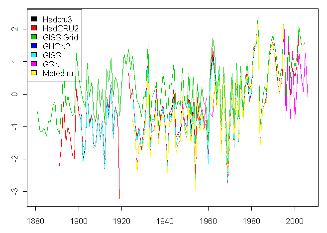
ts.plot(combine[,1:7],col=1:7)#,lwd=c(2,2,1,1,1,1,1),xlab="",ylab="")
legend(1875,2.6,fill=1:7,legend=c("Hadcru3","HadCRU2","GISS Grid","GHCN2","GISS","GSN","Meteo.ru"))

This yields this following spaghetti graph on my machine:
barabi1.gif

Now you’ll have to have installed the ncdf package and to have downloaded three large zipped files. I’ve not tried to include the unzipping of these large files in the programming since it’s probably a get idea to do this manually to be sure that you get it right. The three large files are:

HadCRUT3 – downloaded and unzipped from http://hadobs.metoffice.com/hadcrut3/data/HadCRUT3.nc into “d:/climate/data/jones/hadcrut3/HadCRUT3.nc” #5×5 monthly gridded from CRU

GISS Gridded – downloaded and unzipped from ftp://data.giss.nasa.gov/pub/gistemp/netcdf/calannual-1880-2005.nc into “d:/climate/data/jones/giss/calannual-1880-2005.nc” #2×2 degree annual gridded from GISS

GHCN Station data – # http://www1.ncdc.noaa.gov/pub/data/ghcn/v2/v2.mean.Z #unzipped, read and re-collated into “d:/climate/data/jones/ghcn/v2d.tab” #see this script for the re-collation to the R-object

HadCRUT2 – downloaded from HAdCRU and re-collated into “d:/climate/data/jones/hadcrut2/hadcruv.tab” – I posted up a script to do this some time ago, but this probably needs to be reviewed.

There may very well be some residual references to things on my computer that will need to be ironed out to make the routines fully objective. Let me know if you run into problems.

In the mean-time, you should be able to get useful components working and I hope that this helps people to wade through the gridcell data.

Barabinsk, Russia 57N,ย 77E

I’ve been going through the process of reconciling gridded data and station data in one Russian gridcell. Most of my effort to date has been spent on creating tools for accessing and collating data archives into organized time series formats so that others don’t have to go through the same trials and tribulations of sorting out oddball data formats and can improve their analyses on their own gridcells if they want. I’ll post a variety of read scripts up in a day or two. I’ve been working with the gridcell 57.5N and 77.5E primarily because it happened to be adjacent to the Tarko-Sale gridcell, which I had posted on previously. It also appears to include only one station so reconciliation is easier and to have several archives that can be cross-checked.

I report here on 4 archives with station data on Barabinsk (GHCN v2, GISS, GSN, meteo.ru), two of which have daily information (GSN, meteo.ru). There are some other archives – NDP040, NDP048, an early Jones version – which I’ll try to create tools for as well. I also report on 3 gridded versions – HadCRU3, HadCRU2, GISS. Other gridded versions include CRUTEM3 and CRUTEM2 and some early Jones versions.

There are puzzles surrounding not simply the gridded data, but even the GHCN v2 station data. The GHCNv2 archived version ends in 1989, but the GSN version – which reconciles to the GHCN version during their overlap, continues to the present, but is not incorporated in GHCN. The HadCRU3 gridded version ends in 1989 matching GHCN v2 except for 3 oddball monthly values in 2005; however HadCRU2 went to 2002 (and started 10 years earlier than HadCRU3.) It appears to use the updated Barabinsk information available at GSN, but ignored in HadCRU3. The GISS gridded version diverges from both.

At this point, I have no particular conclusions about this aspect of temperature history; I am merely trying to look at available information in an organized way. I will observe that these gridded temperature calculations are as much an accounting exercise as anything else. As an accounting exercise, audit trails “matters”. Thus regardless of whether or not any of this “matters” for policy, it is hard to get a favorable impression of how the audit trails are organized. Continue reading

Reading GISS Station Data

GISS has a large collection of station data, both adjusted and unadjusted. Unlike many data archives, GISS do not permit you to either extract the entire data set from a single archive or from permanent individual files. You can obtain digital data for individual stations, but you have to go through a laborious process of manually clicking on several links for each station, then copying a file to a text file and then working with the saved file.

Until now.

CA reader Nicholas, who had previously developed a nice method for reading for reading zip files, has provided me with a very pretty method of reading GISS station data into R objects. Some of his programming techniques were new to me and I thought that it might be of interest to other readers, especially since some of his methods can be modified to do slightly different tasks.

Don’t try to cut-and-paste code from the WordPress version here. Use an ASCII version here. I’m going to massage this a little and will make up a collection of similar retrieval scripts (which I’ll link here as well.)
Continue reading