The Marcott-Shakun Dating Service

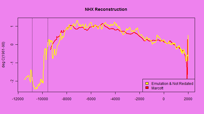
Marcott, Shakun, Clark and Mix did not use the published dates for ocean cores, instead substituting their own dates. The validity of Marcott-Shakun re-dating will be discussed below, but first, to show that the re-dating “matters” (TM-climate science), here is a graph showing reconstructions using alkenones (31 of 73 proxies) in Marcott style, comparing the results with published dates (red) to results with Marcott-Shakun dates (black). As you see, there is a persistent decline in the alkenone reconstruction in the 20th century using published dates, but a 20th century increase using Marcott-Shakun dates. (It is taking all my will power not to make an obvious comment at this point.)
alkenone-comparison
Figure 1. Reconstructions from alkenone proxies in Marcott style. Red- using published dates; black- using Marcott-Shakun dates.

Marcott et al archived an alkenone reconstruction. There are discrepancies between the above emulation and the archived reconstruction, a topic that I’ll return to on another occasion. (I’ve tried diligently to reconcile, but am thus far unable. Perhaps due to some misunderstanding on my part of Marcott methodology, some inconsistency between data as used and data as archived or something else.) However, I do not believe that this matters for the purposes of using my emulation methodology to illustrate the effect of Marcott-Shakun re-dating.

ALkenone Core Re-dating

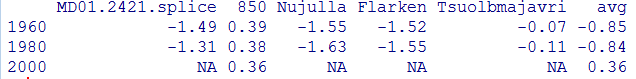
The table below summarizes Marcott-Shakun redating for all alkenone cores with either published end-date or Marcott end-date being less than 50 BP (AD1900). I’ve also shown the closing temperature of each series (“close”) after the two Marcot re-centering steps (as I understand them).
alkenone core redating table

The final date of the Marcott reconstruction is AD1940 (BP10). Only three cores contributed to the final value of the reconstruction with published dates ( “pubend” less than 10): the MD01-2421 splice, OCE326-GGC30 and M35004-4. Two of these cores have very negative values. Marcot et al re-dated both of these cores so that neither contributed to the closing period: the MD01-2421 splice to a fraction of a year prior to 1940, barely missing eligibility; OCE326-GGC30 is re-dated 191 years earlier – into the 18th century.

Re-populating the closing date are 5 cores with published coretops earlier than AD10, in some cases much earlier. The coretop of MD95-2043, for example, was published as 10th century, but was re-dated by Marcott over 1000 years later to “0 BP”. MD95-2011 and MD-2015 were redated by 510 and 690 years respectively. All five re-dated cores contributing to the AD1940 reconstruction had positive values.

In a follow-up post, I’ll examine the validity of Marcott-Shakun redating. If the relevant specialists had been aware of or consulted on the Marcott-Shakun redating, I’m sure that they would have contested it.

Jean S had observed that the Marcott thesis had already described a re-dating of the cores using CALIB 6.0.1 as follows:

All radiocarbon based ages were recalibrated with CALIB 6.0.1 using INTCAL09 and its protocol (Reimer, 2009) for the site-specific locations and materials. Marine reservoir ages were taken from the originally published manuscripts.

The SI to Marcott et al made an essentially identical statement (pdf, 8):

The majority of our age-control points are based on radiocarbon dates. In order to compare the records appropriately, we recalibrated all radiocarbon dates with Calib 6.0.1 using INTCAL09 and its protocol (1) for the site-specific locations and materials. Any reservoir ages used in the ocean datasets followed the original authors’ suggested values, and were held constant unless otherwise stated in the original publication.

However, the re-dating described above is SUBSEQUENT to the Marcott thesis. (I’ve confirmed this by examining plots of individual proxies on pages 200-201 of the thesis. End dates illustrated in the thesis correspond more or less to published end dates and do not reflect the wholesale redating of the Science article.

I was unable to locate any reference to the wholesale re-dating in the text of Marcott et al 2013. The closest thing to a mention is the following statement in the SI:

Core tops are assumed to be 1950 AD unless otherwise indicated in original publication.

However, something more than this is going on. In some cases, Marcott et al have re-dated core tops indicated as 0 BP in the original publication. (Perhaps with justification, but this is not reported.) In other cases, core tops have been assigned to 0 BP even though different dates have been reported in the original publication. In another important case (of YAD061 significance as I will later discuss), Marcott et al ignored a major dating caveat of the original publication.

Examination of the re-dating of individual cores will give an interesting perspective on the cores themselves – an issue that, in my opinion, ought to have been addressed in technical terms by the authors. More on this in a forthcoming post.

The moral of today’s post for ocean cores. Are you an ocean core that is tired of your current date? Does your current date make you feel too old? Or does it make you feel too young? Try the Marcott-Shakun dating service. Ashley Madison for ocean cores. Confidentiality is guaranteed.

How Marcottian Upticks Arise

I’m working towards a post on the effect of Marcott re-dating, but first I want to document some points on the methodology of Marcott et al 2013 and to remove some speculation on the Marcott upticks, which do not arise from any of the main speculations.

In the graphic below, I’ve plotted Marcott’s NHX reconstruction against an emulation (weighting by latitude and gridcell as described in script) using proxies with published dates rather than Marcott dates. (I am using this version because it illustrates the uptick using Marcott methodology. Marcott re-dating is an important issue that I will return to.) The uptick in the emulation occurs in 2000 rather than 1940; the slight offset makes it discernible for sharp eyes below.

emulation -NH
Figure 1. Marcott NHX reconstruction (red) versus emulation with non-redated proxies (yellow). The dotted lines at the left show the Younger Dryas. Marcott began their reported results shortly after the rapid emergence from the Younger Dryas, which is not shown in the graphics.

I have consistently discouraged speculation that the Marcott uptick arose from splicing Mannian data or temperature data. I trust that the above demonstration showing a Marcottian uptick merely using proxy data will put an end to such speculation.

The other “explanation” is that the uptick results from high-frequency swings in individual proxies. Marcott’s email to me encouraged such speculation. However, this is NOT what causes the uptick. Below I show the series that contribute to the NHX weighted average before and after the uptick. The proxy values shown below have been re-centered to reflect Marcott recentering: (1) by -0.66 deg C to reflect the re-centering from mid-Holocene to 500-1450AD; (2) by -0.08 deg C to match the observed mean of Marcottian reconstructions in 500-1450 AD.

Readers will observe that there are 6 contributing series in the second-last step, of which 5 are negative, some strongly. Their weighted average is negative (not quite as negative as the penultimate Marcott value in 1920, but you see the effect.) Only one series is present in the final step, one that, after the two rescaling steps, is slightly positive. Thus, the uptick. None of the contributing series have sharp high-frequency: their changes are negligible. Ironically, the one continuing series (Lake 850) actually goes down a little in the period of the uptick.

excerpt nh unredated

Marcottian uptricks upticks arise because of proxy inconsistency: one (or two) proxies have different signs or quantities than the larger population, but continue one step longer. This is also the reason why the effect is mitigated in the infilled variation. In principle, downticks can also occur – a matter that will be covered in my next post which will probably be on the relationship between Marcottian re-dating and upticks.

I have been unable to replicate some of the recent features of the Marcott zonal reconstructions. I think that there may be some differences in some series between the data as archived and as used in their reported calculations, though it may be a difference in methodology. More on this later.

CG3: The Gold Medalist

bolt_mann Last summer during the London Olympics, Josh had some fun with the “Climate Olympics”, with Mann at left in the iconic gold medal pose of Usain Bolt, the famous runner.

Little did we know that during an earlier Olympics, Jones was disappointed at being silver medalist in statistical abuse – to gold medalist Mann. CG3 1093965453:

date: Tue Aug 31 11:17:33 2004
from: Phil Jones

subject: Fwd: On the Role of Statistics in Climate Research, Tim Lambert, Phil Jones et al?
to: Rasmus Benestad

Rasmus and Mike,

In the email below, Mike seems to have won the gold medal for statistical abuse and I have the silver. I seemed to have tried too hard to explain my techniques. I tried really hard to get the gold medal – Mike has a degree in maths/stats ! I’ll have to redeem myself in AR4 and switch the places for the 2008 Olympiad – the AR4 coming out in 2007 should put me well in the lead.

I clearly didn’t allow for the knowledge of the judges – I think I’ll appeal!

Cheers
Phil

The category remains hotly contested, with many new contestants. Jones, whatever his other sins, has tended to use fairly simple methods and I find it hard to picture him maintaining a spot on the podium. Mann, of course, has a repertoire of upside-down techniques that are highly regarded by climate referees and which make it very difficult for new contestants to seize the gold medal.

Marcott’s Zonal Reconstructions

I’m going to do a detailed post on my diagnosis of the Marcott uptick, but before I do so, I want to comment on the reconstructions for NH and SH extratropics, neither of which have attracted sufficient notice though both are very remarkable. In a substantive sense, because orbital changes have different effects on NH and SH, the difference between NHX and SHX proxies is a source of substantive interest and is what ought to have been reported on.

In the running text, Marcott et al had emphasized that their reconstruction was “indistinguishable within uncertainty”. This was illustrated in their Figure 1E, which showed the Mann08 GLB and NH reconstructions (which of several versions is not denoted in the caption), Moberg 2005 (NH) and the Wahl-Ammann version of MBH98 (NH).

Our global temperature reconstruction for the past 1500 years is indistinguishable within uncertainty from the Mann et al. (2) reconstruction… This similarity confirms that published temperature reconstructions of the past two millennia capture long-term variability, despite their short time span (3, 12, 13).

The zonal (NHX, SHX and tropics) reconstructions were illustrated in Marcott Figure 2I,J,K, but Marcott et al conspicuously did not compare their zonal reconstructions with previous NH and SH reconstructions, instead comparing them to proxies often considered to be precipitation proxies. In their text, they stated:

Trends in regional temperature reconstructions show strong similarities with high-resolution precipitation records, consistently associating greater warmth with greater wetness (Fig. 2, H to J). For example, extratropical Northern Hemisphere mid-to- high–latitude temperature correlates well with records of Asian monsoon intensity (14, 15 -Dongge O18) and the position of the Atlantic intertropical convergence zone (16 – Cariaco) (Fig. 2H), tropical temperatures track precipitation proxies from speleothems in Borneo (17) and Indonesia (18) (Fig. 2I), and extratropical Southern Hemisphere temperatures parallel speleothem proxies of precipitation and temperature from South Africa (19) and South America (20) that are independent of our reconstruction

Their decision not to compare their reconstruction to popular hemispherical versions was a curious one and I’ve remedied this apparent oversight below.

Northern Hemisphere
First here is a comparison of the Marcott NH Extratropic reconstruction with the Moberg 2005 reconstruction (which Marcott et al showed in connection with their GLB reconstruction). I suspect that some readers will not find these two series to be “remarkably similar” (TM- climate science). (For greater certainty, Marcott et al did not say that these two series were “remarkably similar”, he said that the Moberg NH reconstruction was similar to his GLB reconstruction, but omitted any direct comparison with his NHX reconstructions.

moberg-vs-marcott
Figure 1. Moberg NH versus Marcott et al NHX. Red dot shows 1990-2010 average HadCRU temperature. Dotted vertical black line at 1890 is period after which reconstruction already admitted to be “not robust”.

Next here is a comparison of the Marcott NHX reconstruction with two Mann reconstructions: the Mann 2008 NH EIV iHAD variation (which in effect splices temperature from 1850 on) and the MBH NHX version (extracted from Briffa et al 2001 SI). I am not persuaded that Marcott’s NHX reconstruction is “indistinguishable within uncertainty” from the corresponding NH reconstructions, making one wonder why the GLB reconstruction is are supposedly “indistinguighable within uncertainty”.

mann-vs-marcott
Figure 2. Marcott NHX versus M08 NH EIV iHAD and MBH98-99 NHX (from Briffa et al 2001). As Figure 1.

Southern Hemisphere
In the figure below, I’ve first compared the Marcott et al SHX reconstruction to the SH reconstruction of Mann and Jones 2003. After readers recover from their awe at the remarkable similarity (TM-climate science) between the two reconstructions, they will note that the Marcott reconstruction began a pronounced and dramatic increase in the 18th century and reached its maximum in AD1900, which, in their Northern Hemisphere reconstruction, was the coldest year since the LGM. Marcott’s estimated AD1900 temperatures in SHX were much higher than even recent temperatures (1990-2010 HadCRU SH average denoted by red dot.)

mj03-vs-marcott_SH
Figure 3. Marcott SHX vs Mann and Jones 2003 SH.

Finally, here is a comparison of Mann 2008 SH EIV-CRU and CPS-CRU versus Marcott. There are important inconsistencies between Mannian EIV and CPS results, improving the odds of matching at least one of them. (Why anyone would regard Mannian EIV as an “improvement” on anything is a continuing source of puzzlement to me, but that is another day’s story.) Even doubling the odds of a match, I find the correspondence between the Mannian and Marcottian version to be underwhelming, though perhaps not so underwhelming as to preclude them being “remarkably similar TM-climate science”.

mann-vs-marcott_SH

I will return to details of the uptick later. For now, I’ll close with this graphic showing the NHX and SHX reconstructions against the GLB reconstruction shown as the Marcott base. While one expects a difference between NHX and SHX in the Holocene, the remarkable difference between NHX and SHX not just in the 20th century, but in the 19th century is a source of considerable interest. According to Marcott, NHX temperatures increased by 1.9 deg C between 1920 and 1940, a surprising result even for the most zealous activists. But for the rest of us, given the apparent resiliency of our species to this fantastic increase over a mere 20 years, it surely must provide a small measure of hope for resiliency in the future.

figure1B-loop
Figure ^. SHX (blue) and NHX (red) shown against global. Third zone (tropics) not shown only to emphasize contrast. Full spaghetti would include a third zone.

No Uptick in Marcott Thesis

Reader ^ drew our attention to Marcott’s thesis (see chapter 4 here. Marcott’s thesis has a series of diagrams in an identical style as the Science article. The proxy datasets are identical.

However, as Jean S alertly observed, the diagrams in the thesis lack the closing uptick of the Science. Other aspects of the modern period also differ dramatically.

Here is Figure 1C of the Science article.

figure 1C

Now here is the corresponding diagram from the thesis (Figure 4.3a):
thesis-short1

The differences will be evident to readers. In addition to the difference in closing uptick, important reconstruction versions were at negative values in the closing portion of the thesis graphic, while they were at positive values in the closing portion of the Science graphic.

I wonder what accounts for the difference.

A similar phenomenon occurs with the simulation diagram, that has been widely distributed as Stick support. Here is a blowup of the recent portion in Sciencemag:
SI figure3 simulation blowup

Here is a corresponding blowup from the thesis.
thesis simulation blowup

Marcott Mystery #1

Marcott et al 2013 has received lots of publicity, mainly because of its supposed vindication of the Stick. A number of commenters have observed that they are unable to figure out how Marcott got the Stick portion of his graph from his data set. Add me to that group.

The uptick occurs in the final plot-point of his graphic (1940) and is a singleton. I wrote to Marcott asking him for further details of how he actually obtained the uptick, noting that the enormous 1920-to-1940 uptick is not characteristic of the underlying data. Marcott’s response was unhelpful: instead of explaining how he got the result, Marcott stated that they had “clearly” stated that the 1890-on portion of their reconstruction was “not robust”. I agree that the 20th century portion of their reconstruction is “not robust”, but do not feel that merely describing the recent portion as “not robust” does full justice to the issues. Nor does it provide an explanation.

The uptick problems are even more pronounced in the zonal temperature reconstructions (NH and SH extratropics on which I will be posting) and in the reconstructions from individual proxies (alkenone, Mg/Ca). In today’s post, I’ll illustrate the uptick problem from the alkenone temperature stack on the premise that there are fewer moving parts in the alkenone reconstruction and therefore this will facilitate diagnosis of the uptick mystery. Continue reading

More News from RC/FOIA

Tom Nelson and Bishop Hill have released the following letter from Mr FOIA. I was one of several people who received the following letter:

It’s time to tie up loose ends and dispel some of the speculation surrounding the Climategate affair.

Indeed, it’s singular “I” this time. After certain career developments I can no longer use the papal plural 😉

If this email seems slightly disjointed it’s probably my linguistic background and the problem of trying to address both the wider audience (I expect this will be partially reproduced sooner or later) and the email recipients (whom I haven’t decided yet on).

The “all.7z” password is [deracted] DO NOT PUBLISH THE PASSWORD. Quote other parts if you like.

Releasing the encrypted archive was a mere practicality. I didn’t want to keep the emails lying around.

I prepared CG1 & 2 alone. Even skimming through all 220.000 emails would have taken several more months of work in an increasingly unfavorable environment.

Dumping them all into the public domain would be the last resort. Majority of the emails are irrelevant, some of them probably sensitive and socially damaging.

To get the remaining scientifically (or otherwise) relevant emails out, I ask you to pass this on to any motivated and responsible individuals who could volunteer some time to sift through the material for eventual release.

Filtering\redacting personally sensitive emails doesn’t require special expertise.

I’m not entirely comfortable sending the password around unsolicited, but haven’t got better ideas at the moment. If you feel this makes you seemingly “complicit” in a way you don’t like, don’t take action.

I don’t expect these remaining emails to hold big surprises. Yet it’s possible that the most important pieces are among them. Nobody on the planet has held the archive in plaintext since CG2.

That’s right; no conspiracy, no paid hackers, no Big Oil. The Republicans didn’t plot this. USA politics is alien to me, neither am I from the UK. There is life outside the Anglo-american sphere.

If someone is still wondering why anyone would take these risks, or sees only a breach of privacy here, a few words…

The first glimpses I got behind the scenes did little to garner my trust in the state of climate science — on the contrary. I found myself in front of a choice that just might have a global impact.

Briefly put, when I had to balance the interests of my own safety, privacy\career of a few scientists, and the well-being of billions of people living in the coming several decades, the first two weren’t the decisive concern.

It was me or nobody, now or never. Combination of several rather improbable prerequisites just wouldn’t occur again for anyone else in the foreseeable future. The circus was about to arrive in Copenhagen. Later on it could be too late.

Most would agree that climate science has already directed where humanity puts its capability, innovation, mental and material “might”. The scale will grow ever grander in the coming decades if things go according to script. We’re dealing with $trillions and potentially drastic influence on practically everyone.

Wealth of the surrounding society tends to draw the major brushstrokes of a newborn’s future life. It makes a huge difference whether humanity uses its assets to achieve progress, or whether it strives to stop and reverse it, essentially sacrificing the less fortunate to the climate gods.

We can’t pour trillions in this massive hole-digging-and-filling-up endeavor and pretend it’s not away from something and someone else.

If the economy of a region, a country, a city, etc. deteriorates, what happens among the poorest? Does that usually improve their prospects? No, they will take the hardest hit. No amount of magical climate thinking can turn this one upside-down.

It’s easy for many of us in the western world to accept a tiny green inconvenience and then wallow in that righteous feeling, surrounded by our “clean” technology and energy that is only slightly more expensive if adequately subsidized.

Those millions and billions already struggling with malnutrition, sickness, violence, illiteracy, etc. don’t have that luxury. The price of “climate protection” with its cumulative and collateral effects is bound to destroy and debilitate in great numbers, for decades and generations.

Conversely, a “game-changer” could have a beneficial effect encompassing a similar scope.

If I had a chance to accomplish even a fraction of that, I’d have to try. I couldn’t morally afford inaction. Even if I risked everything, would never get personal compensation, and could probably never talk about it with anyone.

I took what I deemed the most defensible course of action, and would do it again (although with slight alterations — trying to publish something truthful on RealClimate was clearly too grandiose of a plan ;-).

Even if I have it all wrong and these scientists had some good reason to mislead us (instead of making a strong case with real data) I think disseminating the truth is still the safest bet by far.

Big thanks to Steve and Anthony and many others. My contribution would never have happened without your work (whether or not you agree with the views stated).

Oh, one more thing. I was surprised to learn from a “progressive” blog, corroborated by a renowned “scientist”, that the releases were part of a coordinated campaign receiving vast amounts of secret funding from shady energy industry groups.

I wasn’t aware of the arrangement but warmly welcome their decision to support my project. For that end I opened a bitcoin address: [redacted for now].

More seriously speaking, I accept, with gratitude, modest donations to support The (other) Cause. The address can also serve as a digital signature to ward off those identity thefts, which are part of climate scientists’ repertoire of tricks these days.

Keep on the good work. I won’t be able to use this email address for long so if you reply, I can’t guarantee reading or answering. I will several batches, to anyone I can think of.

Over and out.

Mr. FOIA

An Interesting Graphic in the Esper et al 2012 SI

Rob Wilson (by email) has drawn my attention to the SI to Esper et al 2012 SI, which contains the following diagram relevant to late Holocene treeline changes.

esper 2012 SI treeline
Figure 1. From Esper et al 2012 SI. Continue reading

Mike’s AGU Trick

There has been considerable recent discussion of the fact that observations have been running cooler than models – see, for example, Lucia’s discussion of IPCC AR5 SOD Figure 9.8 (see here). However, Michael Mann at AGU took an entirely different line. Mann asserted that observations were running as hot or hotter than models. Mann’s assertion was taken even further by Naomi Oreskes, who asserted that climate models were under-estimating relative to observations. Oreskes squarely placed the blame for the supposed underestimates on climate skeptics.

In today’s post, I’ll look closely at the illustration in Mann’s AGU presentation, an illustration that gave an entirely different impression than the figure in the IPCC draft report. The reason for the difference can be traced to what I’ve termed here as “Mike’s AGU Trick”. Continue reading

More on Acton’s “Investigation”

More news on Acton’s supposed “investigation” of the deletion of emails. New documents show that Acton did not even meet with Briffa or Jones in his supposed “investigation” of the deletion of emails. Acton sent Briffa a letter asking him whether he had “knowingly” deleted emails subject to FOI. Briffa wrote back that he hadn’t. That appears to be the entire extent of Acton’s “investigation”. Sort of like Penn State.

Also see Bishop Hill on this story here.
Continue reading